
우리는 그 동안 line bundle을 활용하여 다양한 invariant를 생각할 수 있다는 것을 확인하였다. 가령 §선다발과 벡터다발에서 우리는 line bundle \(\mathcal{L}\)의 global section space \(\Gamma(X, \mathcal{L})\)을 정의하였다. 특히 §선형계, ⁋명제 7에서는 이 차원이 complete linear system의 dimension, 나아가 variety의 projective embedding을 결정하는 핵심적 역할을 한다는 것을 살펴보았다.
우리는 지금까지 기하적 직관을 위해 주로 line bundle의 언어를 사용하였으나, §표준선다발, ⁋정의 1 직후에 살펴보았듯 line bundle의 section sheaf를 생각하면 이는 근본적으로는 sheaf의 언어로 바꾸어 쓸 수 있다. 이번 글에서 우리는 sheaf cohomology의 개념을 정의한다.
Derived Functor로서의 정의
Sheaf가 위상공간의 모든 정보들을 체계적으로 기술할 수 있는 도구임에 반해, 지금까지의 이야기에서 sheaf가 전면으로 등장한 것은 §선형계에서 global section space \(\Gamma(X, \mathcal{L})\)이 complete linear system의 projective embedding을 결정한다는 것을 살펴볼 때 뿐이었다.
그러나 global section만이 우리의 관심사라면, 굳이 sheaf를 생각할 필요 없이 global section functor만 생각했어도 될 것이다. 실제로 global section functor는 sheaf가 갖고 있는 정보를 모두 담고 있는 것이 아니다. 예를 들어 global section functor
\[\Gamma(X, -): \QCoh(X) \to \Vect_\mathbb{K}; \qquad \mathcal{F} \mapsto \mathcal{F}(X)\]를 생각하자. 우리가 §표준선다발, ⁋정의 1에서 quasi-coherent sheaf를 정의할 때의 motivation은 vector bundle들의 category \(\Bun(X)\)가 abelian category가 아니므로, kernel과 cokernel을 추가하는 더 넓은 category를 생각하는 것이었고, 그러한 관점에서 \(\QCoh(X)\)가 abelian category가 된다는 것은 놀라운 일은 아니다. 1
만일 \(\Gamma(X,-)\)가 어떠한 정보도 잃어버리지 않는다면, 이 functor는 exact functor여야 할 것이다. 즉, (quasi-coherent) sheaf들의 short exact sequence
\[0 \to \mathcal{F}' \to \mathcal{F} \to \mathcal{F}'' \to 0\]가 주어졌을 때, 이를 \(\Gamma(X,-)\)를 타고 옮긴 것 또한 short exact sequence가 되어야 할 것이다. 그러나 이 functor는 left exact functor밖에 되지 않는다. 즉,
\[0 \to \Gamma(X, \mathcal{F}') \to \Gamma(X, \mathcal{F}) \to \Gamma(X, \mathcal{F}'')\]의 exactness는 보장되지만 surjection
\[\Gamma(X, \mathcal{F}) \to \Gamma(X, \mathcal{F}'') \to 0\]은 일반적으로 보장되지 않는다. 구체적인 예시를 위해 Euler sequence
\[0 \to \Omega^1_{\mathbb{P}^n} \to \mathcal{O}_{\mathbb{P}^n}(-1)^{\oplus(n+1)} \to \mathcal{O}_{\mathbb{P}^n} \to 0\]를 생각하자. (§표준선다발, ⁋명제 7) 이 short exact sequence에 \(\Gamma(\mathbb{P}^n, -)\)를 적용하면
\[0 \to \Gamma(\mathbb{P}^n, \Omega^1_{\mathbb{P}^n}) \to \Gamma(\mathbb{P}^n, \mathcal{O}_{\mathbb{P}^n}(-1)^{\oplus(n+1)}) \to \Gamma(\mathbb{P}^n, \mathcal{O}_{\mathbb{P}^n})\]를 얻는다. 그런데 §선다발과 벡터다발, ⁋예시 16에서 살펴본 것처럼 \(\mathcal{O}_{\mathbb{P}^n}(-1)\)의 global section은 0뿐이므로
\[\Gamma(\mathbb{P}^n, \mathcal{O}_{\mathbb{P}^n}(-1)^{\oplus(n+1)}) = 0\]이지만, \(\Gamma(\mathbb{P}^n, \mathcal{O}_{\mathbb{P}^n})=\mathbb{K}\)이므로 오른쪽 부분의 surjectivity가 성립할 수 없다.
이를 해결하기 위한 표준적인 방법은 right derived functor를 생각하는 것이다. ([호몰로지 대수학] §유도함자, ⁋정의 9). 구체적으로, \(\lMod{A}\)는 enough injective를 가지므로, 이들을 이어붙여 \(\QCoh(X)\)도 충분한 injective object가 존재하는 것을 보일 수 있으므로 임의의 quasi-coherent sheaf \(\mathcal{F}\)는 항상 injective resolution \(\mathcal{I}^\bullet\)을 가지고, 이로부터 다음의
\[0 \to \Gamma(X, \mathcal{I}^0) \to \Gamma(X, \mathcal{I}^1) \to \Gamma(X, \mathcal{I}^2) \to \cdots\]를 통해 다음의 sheaf cohomology를 정의할 수 있다.
정의 1 Variety \(X\) 위의 quasi-coherent sheaf \(\mathcal{F}\)에 대하여, \(i\)번째 sheaf cohomology \(H^i(X, \mathcal{F})\)를
\[H^i(X, \mathcal{F}) = \frac{\ker(\Gamma(X, \mathcal{I}^i) \to \Gamma(X, \mathcal{I}^{i+1}))}{\im(\Gamma(X, \mathcal{I}^{i-1}) \to \Gamma(X, \mathcal{I}^i))}\]으로 정의한다. 여기서 \(\mathcal{I}^\bullet\)은 \(\mathcal{F}\)의 injective resolution이다.
더 일반적으로, \(X\) 위의 임의의 sheaf에 대해서도 stalk별로 injective object를 잡은 후 sheafification을 취해주면 \(\Sh(X)\)가 enough injective를 갖는다는 것을 보일 수 있으나, 우리의 주된 관심은 항상 quasi-coherent sheaf 뿐이므로 category \(\QCoh(X)\)로 우리의 관심을 제한한다.
이것이 \(\mathcal{I}^\bullet\)의 선택에 무관한 것 등등은 모두 homological algebra의 표준적인 논증으로부터 따라온다.
우리는 앞서 global section space \(\Gamma(X, \mathcal{L})\)을 소개하며 이 공간의 또 다른 대중적인 표기 중 하나가 \(H^0(X, \mathcal{L})\)이라고 하였는데, 이 표기법이 바로 위의 정의로부터 정당화됨을 안다.
다음 명제 또한 homological algebra로부터 바로 따라나오는 표준적인 명제이다. ([호몰로지 대수학] §유도함자, ⁋명제 8)
명제 2 Sheaf의 short exact sequence
\[0 \to \mathcal{F}' \to \mathcal{F} \to \mathcal{F}'' \to 0\]에 대하여, long exact sequence
\[0 \to H^0(X, \mathcal{F}') \to H^0(X, \mathcal{F}) \to H^0(X, \mathcal{F}'') \xrightarrow{\delta} H^1(X, \mathcal{F}') \to \cdots\]이 존재한다. 여기서 \(\delta\)는 connecting homomorphism이다.
Čech Cohomology
정의 1는 sheaf cohomology의 정의로서는 엄밀하지만, injective resolution을 명시적으로 구성하는 것은 일반적으로 매우 어렵다. 따라서 실제 계산에서는 다른 관점에서 cohomology를 정의하는 Čech approach를 사용한다.
직관적으로 Čech cohomology \(\check{H}^i(X, \mathcal{F})\)는 국소적인 정보의 gluing의 실패를 측정하는 도구이다. 즉, \(\check{H}^0(X, \mathcal{F})\)는 정확하게 global section space이며, \(\check{H}^1(X, \mathcal{F})\)는 local section들을 붙여서 global section을 얻어내는 과정이 얼마나 실패하는지를 알려준다. 이를 엄밀하게 정의하기 위해 다음부터 시작한다.
정의 3 위상공간 \(X\)의 open cover \(\mathcal{U} = \{U_i\}_{i \in I}\)와 sheaf \(\mathcal{F}\)가 주어졌다 하고, \(I\) 위의 total order \(<\)를 임의로 고정하자. 그럼 이들 데이터의 Čech complex체흐 복합체 \(C^\bullet(\mathcal{U}, \mathcal{F})\)는 다음과 같이 정의된다.
\[\check{C}^p(\mathcal{U}, \mathcal{F}) = \prod_{i_0 < \cdots < i_p} \mathcal{F}(U_{i_0} \cap \cdots \cap U_{i_p})\]이 때, coboundary map \(d: \check{C}^p \to \check{C}^{p+1}\)은 다음의 식
\[(d\alpha)_{i_0 \cdots i_{p+1}} = \sum_{k=0}^{p+1} (-1)^k \alpha_{i_0 \cdots \hat{i_k} \cdots i_{p+1}}\vert_{U_{i_0}\cap \cdots \cap U_{i_{p+1}}}\]으로 정의된다. 여기서 \(\hat{i_k}\)는 index \(i_k\)를 생략한다는 의미이다.
Sheaf cohomology에서와 마찬가지로, 이 정의는 임의의 sheaf에 대해서도 말이 되지만, 우리는 주로 \(\QCoh(X)\)만을 신경쓴다.
이 정의가 잘 정의되기 위해서는, 즉, \(\check{C}^\bullet(\mathcal{U}, \mathcal{F})\)이 실제로 complex가 되기 위해서는 coboundary map이 실제로 coboundary map이 되어야 한다. 즉 \(d^2=0\)이어야 한다. 이는 위의 식을 전개해보면 부호 차이로부터 직접 확인할 수 있다. 결론적으로 \(\check{C}^\bullet(\mathcal{U}, \mathcal{F})\)는 cochain complex이며, 따라서 다음을 정의할 수 있다.
정의 4 위의 데이터가 정의하는 Čech cohomology체흐 코호몰로지 \(\check{H}^p(\mathcal{U}, \mathcal{F})\)를 Čech complex의 cohomology
\[\check{H}^p(\mathcal{U}, \mathcal{F}) = H^p(\check{C}^\bullet(\mathcal{U}, \mathcal{F}))\]로 정의한다.
우리는 앞서 Čech cohomology가 gluing의 실패를 측정해주는 도구라 하였는데, 이는 coboundary map에 담겨있다. Coboundary map의 직관적 의미를 낮은 차원 \(p = 0, 1\)에서 확인해보자.
예시 5 (\(p = 0\)) Čech complex의 정의에 의하여 \(\check{C}^0(\mathcal{U}, \mathcal{F}) = \prod_i \mathcal{F}(U_i)\)이고, \(\check{C}^0\)에서 \(\check{C}^1\)로의 coboundary map은
\[(ds)_{ij} = s_j\vert_{U_i \cap U_j} - s_i\vert_{U_i \cap U_j}\]이다. 따라서
\[\check{H}^0(\mathcal{U}, \mathcal{F}) = \ker(d: \check{C}^0 \to \check{C}^1) = \left\{(s_i) \in \prod_i \mathcal{F}(U_i) \mid s_i\vert_{U_i \cap U_j} = s_j\vert_{U_i \cap U_j} \text{ for all } i, j\right\}\]이다. Sheaf의 gluing condition ([위상수학] §층, ⁋정의 1)에 의해 이러한 section들의 family는 정확히 \(X\) 전체 위에서의 section, 즉 \(\Gamma(X, \mathcal{F})\)와 일치한다. 즉, \(\check{H}^0(\mathcal{U}, \mathcal{F}) = H^0(X, \mathcal{F})\)이며 이는 open cover의 선택과 무관하다.
우리는 곧 좋은 상황에서는 위와 같이 Čech cohomology와 sheaf cohomology가 항상 같다는 것을 보일 것이다. 지금은 우선 \(p=1\)인 경우 이것이 어떻게 gluing의 failure를 측정하는지를 보자.
예시 6 (\(p = 1\)) 1-cochain은 각 \(U_i \cap U_j\) 위의 section \(s_{ij} \in \mathcal{F}(U_i \cap U_j)\)들의 모임이며, 1-cocycle은 cocycle condition
\[s_{ij} + s_{jk} = s_{ik} \qquad\text{on}\quad U_i \cap U_j \cap U_k\]을 만족하는 것들이다. 한편 1-coboundary는 0-cochain \((t_i)\)로부터 유도되는 것, 즉 \(s_{ij} = t_j\vert_{U_i \cap U_j} - t_i\vert_{U_i \cap U_j}\)의 꼴이다.
따라서 \(\check{H}^1(\mathcal{U}, \mathcal{F})\)의 nontrivial한 원소는 이들 세 데이터 \(s_{ij}, s_{jk}, s_{ik}\)를 붙이려 할 때 나타나는 차이를 반영하는 것이며, 이것이 위에서 언급한 gluing의 failure라 할 수 있다.
지금까지 우리는 하나의 open cover \(\mathcal{U}\)에 대하여 Čech cohomology \(\check{H}^p(\mathcal{U}, \mathcal{F})\)를 정의하였다. 그러나 일반적으로 서로 다른 open cover는 서로 다른 Čech cohomology를 줄 수 있다. 가령 하나의 열린집합 \(U_0 = X\)으로 이루어진 cover에서는 모든 교집합이 \(X\)이므로 \(\check{H}^p\)가 \(p = 0\)에서만 0이 아닌 값을 갖는다. 더 조밀한 cover를 사용할수록 더 많은 위상적 정보를 포착할 수 있으므로, 우리는 open cover들 사이의 관계를 규명하고 모든 open cover에 대한 정보를 종합할 필요가 있다. 즉,
정의 7 \(X\)의 Čech cohomology를 모든 open cover에 대한 direct limit
\[\check{H}^p(X, \mathcal{F}) = \varinjlim_{\mathcal{U}} \check{H}^p(\mathcal{U}, \mathcal{F})\]으로 정의한다.
위의 논증을 더 간단히 설명하자면, open cover를 점점 더 세밀하게 잡으며 추가되는 cohomology data를 모두 합쳐 이를 \(\check{H}(X, \mathcal{F})\)로 정의하겠다는 의미이다.
일반적으로 정의 7의 \(\check{H}^p(X, \mathcal{F})\)와 정의 1의 \(H^p(X, \mathcal{F})\)가 isomorphic하다는 것은 보장되지 않지만, 다행히 대수기하학에서 등장하는 대부분의 sheaf에 대해서는 둘이 일치한다. 이를 보이기 위해서는 다소 기술적인 것들이 필요하다.
정의 8 Variety \(X\) 위의 sheaf \(\mathcal{F}\)에 대하여, 다음을 정의한다.
- Sheaf \(\mathcal{F}\)가 acyclic이라는 것은 모든 \(i > 0\)에 대해 \(H^i(X, \mathcal{F}) = 0\)인 것이다.
- \(\Sh(X)\)의 injective object \(\mathcal{F}\)를 injective sheaf라 부른다.
- 임의의 열린집합 \(V\subset U\)에 대하여, restriction map \(\mathcal{F}(U) \rightarrow \mathcal{F}(V)\)가 surjective라면 \(\mathcal{F}\)를 flasque sheaf라 부른다.
우리가 cohomology 단계에서 원하는 조건은 물론 첫 번째 조건이다. 우리는 위의 개념들 사이의 관계를 우선 살펴본다.
보조정리 9 Injective sheaf \(\mathcal{F}\)는 flasque이다.
증명
정의에 의해 \(\mathcal{F}\)가 injective라는 것은 임의의 monomorphism \(\mathcal{A} \hookrightarrow \mathcal{B}\)에 대해 \(\Hom_{\Sh(X)}(\mathcal{B}, \mathcal{F}) \to \Hom_{\Sh(X)}(\mathcal{A}, \mathcal{F})\)가 surjective인 것이다. ([호몰로지 대수학] §분해, ⁋정의 1) 이제 임의의 열린집합 \(V \subset U \subset X\)에 대해 restriction \(\mathcal{F}(U) \to \mathcal{F}(V)\)가 surjective임을 보이자.
이 map은 sheaf morphism이 아니라 abelian group들 사이의 morphism이고, 우리가 갖고 있는 도구는 sheaf morphism이므로 이 조건을 sheaf morphism으로 돌려놔야 한다. 이를 위해 open embedding
\[i^U: U \hookrightarrow X,\qquad i^V: V \hookrightarrow X\]그리고 이들의 extension by zero로 얻어지는 sheaf들 \(i^U_!\mathbb{Z}_U, i^V_!\mathbb{Z}_V\)를 도입하자. 여기서 \(\mathbb{Z}_U, \mathbb{Z}_V\)는 각각 constant sheaf들이며, 가정에 의해 \(V \subset U\)이므로 natural한 monomorphism \(i^V_!\mathbb{Z}_V \to i^U_!\mathbb{Z}_U\)가 존재한다.
우선 \(\Hom_{\Sh(X)}(i^U_!\mathbb{Z}_U, \mathcal{F}) \cong \mathcal{F}(U)\)가 성립함을 확인하자. Extension by zero \(i^U_!\)는 restriction \(\mathcal{G} \mapsto \mathcal{G}\vert_U\)의 left adjoint이므로 ([위상수학] §층, ⁋예시 14),
\[\Hom_{\Sh(X)}(i^U_!\mathbb{Z}_U, \mathcal{F}) \cong \Hom_{\Sh(U)}(\mathbb{Z}_U, \mathcal{F}\vert_U)\]이 성립한다. 이제 \(\mathbb{Z}_U\)는 \(U\) 위의 constant sheaf이므로 임의의 열린집합 \(W \subset U\)에 대해 \(\mathbb{Z}_U(W) = \mathbb{Z}\)이며, 모든 section은 상수 함수의 restriction으로 주어진다. 따라서 sheaf morphism \(\varphi: \mathbb{Z}_U \to \mathcal{F}\vert_U\)는 global section의 image \(\varphi_U(1) \in \mathcal{F}(U)\)에 의해 완전히 결정된다. 역으로, 임의의 \(s \in \mathcal{F}(U)\)에 대해 각 \(W \subset U\)에서 \(\mathbb{Z}_U(W) \to \mathcal{F}(W),\; n \mapsto n \cdot s\vert_W\)로 정의하면 well-defined된 sheaf morphism이 된다. 따라서
\[\Hom_{\Sh(U)}(\mathbb{Z}_U, \mathcal{F}\vert_U) \cong \Hom_{\Ab}(\mathbb{Z}, \mathcal{F}(U)) \cong \mathcal{F}(U)\]이 성립한다. 마찬가지로 \(\Hom_{\Sh(X)}(i^V_!\mathbb{Z}_V, \mathcal{F}) \cong \mathcal{F}(V)\)이며, 이제 naturality로부터 이들 사이의 함수가 정확히 restriction \(\mathcal{F}(U)\rightarrow \mathcal{F}(V)\)와 일치함을 안다. 이제 \(\mathcal{F}\)가 injective라는 가정으로부터 이것이 surjective이므로 증명이 완료된다.
보조정리 10 Flasque sheaf \(\mathcal{F}\)는 임의의 open cover \(\mathcal{U}\)에 대해 Čech-acyclic이다. 즉, 모든 \(p > 0\)에 대해 \(\check{H}^p(\mathcal{U}, \mathcal{F}) = 0\)이다.
증명
Augmented Čech complex
\[0 \to \mathcal{F}(U) \xrightarrow{\epsilon} \check{C}^0(\mathcal{U}, \mathcal{F}) \xrightarrow{d^0} \check{C}^1(\mathcal{U}, \mathcal{F}) \xrightarrow{d^1} \cdots\]를 생각하자. 우리가 보여야 할 것은 \(p>0\)에서 이것이 exact라는 것이므로, identity chain map이 nullhomotopic임을 보이면 된다. 이를 위해 각각의 \(p\geq 1\)에 대하여 homotopy operator \(s^p : \check{C}^p(\mathcal{U}, \mathcal{F}) \to \check{C}^{p-1}(\mathcal{U}, \mathcal{F})\)를 명시적으로 구성해야 한다.
이 함수를 정의하기 위해서는 우리는 각각의
\[t=(t_{j_0<\cdots< j_p})\in \check{C}^p(\mathcal{U}, \mathcal{F})\]가 주어졌을 때, \(s^p(t)\)의 각 성분
\[s^p(t)_{j_0<\cdots< j_{p-1}}\]이 어떻게 정의되는지를 설명해야 한다. 본질적으로 우리가 하고 싶은 것은, chain homotopy를 정의하기 위해 항상 그러하듯, index \(i_0\)을 하나 고정한 후 이를 \(j_0<\cdots< j_{p-1}\)에 끼워넣어서 (편의상 \(i_0< j_0<\cdots< j_{p-1}\)이라 하자.)
\[s^p(t)_{j_0<\cdots< j_{p-1}}=t_{i_0< j_0<\cdots < j_{p-1}}\tag{$\ast$}\]으로 정의하는 것이다. 이 때, \(s^p(t)_{j_0<\cdots< j_{p-1}}\)는 그 정의에 의해 \(U_{j_0}\cap\cdots\cap U_{j_{p-1}}\) 위에서의 section이지만, 우변의 \(t_{i_0< j_0<\cdots < j_{p-1}}\)는 그보다 작은 집합 \(U_{i_0}\cap U_{j_0}\cap\cdots\cap U_{j_{p-1}}\)에서의 section임을 주목하자. 일반적인 \(\mathcal{F}\)에 대해서는 이렇게 정의하는 것이 불가능하겠지만, 우리는 \(\mathcal{F}\)가 flasque임을 가정하고 있으므로 항상 이 함수를 extension하여 \(U_{j_0}\cap\cdots\cap U_{j_{p-1}}\)의 section이도록 해줄 수 있으며 식 (\(\ast\)) 또한 이러한 방식으로 이해해야 한다. 그럼 이렇게 정의한 \(s^p\)가 실제로 chain homotopy가 된다는 것은 직접 계산을 해 보면 \(d^{p-1}s^p\)에서 \(i_0\)을 생략해주는 항과, \(s^{p+1}d^p\)에서 \(i_0\)을 넣어주는 항이 부호가 상쇄되어 사라지는 것을 통해 확인할 수 있다.
약간의 기술적인 문제는 우리가 고정한 index \(i_0\)이 \(j_0<\cdots< j_{p-1}\)에 포함되는 경우가 존재할 수 있다는 것이다. 이를 위해 우리는 보편적인 Čech complex 대신 그냥 \(I\)의 \(p+1\)개의 원소 \(i_0,\ldots, i_{p+1}\in I\)로 좌표를 주는 non-alternating Čech complex를 사용한다. 이는 원래의 Čech complex와 quasi-isomorphic하며 따라서 이렇게 우회하는 것이 정당화된다.
정리 11 (Leray) 위상공간 \(X\) 위의 sheaf \(\mathcal{F}\)와 open cover \(\mathcal{U} = \{U_i\}\)에 대하여, 모든 유한한 교집합
\[U_{i_0 \cdots i_p}=U_{i_0}\cap \cdots\cap U_{i_p}\]에서 \(\mathcal{F}\)가 acyclic이면 isomorphism
\[\check{H}^p(\mathcal{U}, \mathcal{F}) \to H^p(X, \mathcal{F})\]이 존재한다.
증명
Sheaf \(\mathcal{F}\)의 injective resolution \(0 \to \mathcal{F} \to \mathcal{I}^0 \to \mathcal{I}^1 \to \cdots\)을 고정하고, double complex
\[K^{p,q} = \check{C}^p(\mathcal{U}, \mathcal{I}^q)\]을 구성하자. 그럼 이 double complex에서 horizontal differential \(d_h\)는 Čech differential이고, vertical differential \(d_v\)는 injective resolution으로부터 오는 differential이다. 이제 [호몰로지 대수학] §스펙트럼 열, ⁋예시 11에서 살펴본 것과 같이, 이 double complex의 total complex \(\Tot(K)^\bullet\)에 정의된 두 filtration
\[F_v^p\Tot(K)^\bullet,\qquad F_h^p\Tot(K)^\bullet\]은 같은 filtered homology \(H^\bullet(\Tot(K))\)로 수렴한다는 것을 안다.
따라서 각각의 filtered complex가 주는 spectral sequence들을 생각하자. 우선 vertical filtration의 경우, \(E_1\) page에서 \(E_1^{p,q} = H^q(K^{p,\bullet})\)이며, \(K^{p,\bullet} = \check{C}^p(\mathcal{U}, \mathcal{I}^\bullet)\)이다. 그런데 \(\check{C}^p(\mathcal{U}, \mathcal{I}^\bullet)\)는, 각 성분을 보면, 각각의 교집합 \(U_{i_0 \cdots i_p}\)로 injective resolution을 제한한 후 cohomology를 취하는 것이므로 \(U_{i_0\cdots i_p}\)에서 \(\mathcal{F}\)의 \(q\)번째 sheaf cohomology와 같고, 따라서 \(\mathcal{F}\)가 acyclic이라는 가정으로부터 모든 \(q>0\)에 대하여 \(E_1^{p,q}=0\)이다. 또, 정의에 의해 \(E_1=\check{C}^p(\mathcal{U}, \mathcal{F})\)이다. 이제 \(E_2\) page는 \(E_1^{p,0}\)의 horizontal differential \(d_h\)에 의한 cohomology로 주어지므로
\[E_2^{p,q}=\begin{cases}\check{H}^p(\mathcal{U}, \mathcal{F})&\text{$q=0$}\\0&\text{otherwise}\end{cases}\]이고 \(E_2^{p,q}=E_\infty^{p,q}\)이다.
이제 horizontal filtration 방향을 보면, \(E_1\) page에서 \(E_1^{p,q} = \check{H}^p(\mathcal{U}, \mathcal{I}^q)\)이다. 그런데 앞서 보조정리 9와 보조정리 10에서 injective sheaf들은 Čech-acyclic임을 보였으므로, \(p > 0\)에서 \(E_1^{p,q} = 0\)이며 남아있는 \(p=0\)에서의 vertical differential에 대한 cohomology는 sheaf cohomology이므로
\[E_2^{p,q}=\begin{cases}H^q(X, \mathcal{F})&\text{$p=0$}\\0&\text{otherwise}\end{cases}\]이고 \(E_2^{p,q}=E_\infty^{p,q}\)이다. 이제 두 spectral sequence는 같은 \(H^\bullet(\Tot(K))\)에 수렴하므로
\[\check{H}^n(\mathcal{U}, \mathcal{F}) \cong H^n(X, \mathcal{F})\]임을 안다.
그렇다면 이 acyclic condition이 얼마나 까다로운지가 우리 직관의 유일한 걸림돌인데, 다행히도 이는 생각보다 널널한 조건이다.
명제 12 Affine variety \(X\) 위의 quasi-coherent sheaf \(\mathcal{F} = \widetilde{M}\)에 대하여, \(H^i(X, \mathcal{F}) = 0\)이 모든 \(i > 0\)에 대해 성립한다.
이에 대한 증명은, \(X\)의 coordinate ring을 \(A\)라 할 때, \(\lMod{A}\) 카테고리에서 \(M\)의 injective resolution \(I^\bullet\)을 찾으면 이것이 (\(\QCoh(X)\)에서의 resolution인) \(\widetilde{I^\bullet}\)을 주며, 이 때 injective module이 주는 sheaf는 항상 flasque이고, 따라서 acyclic이기 때문이다.
이제 임의의 variety \(X\)와 그 위에 정의된 quasi-coherent sheaf \(\mathcal{F}\)를 생각하고, \(\mathcal{F}\)의 affine open cover \(\mathcal{U}\)가 주어졌다 하자. 그럼 이들 데이터가 정리 11의 전제조건을 만족하기 위해서는 \(\mathcal{U}\)의 임의의 유한한 교집합이 다시 affine이어야 하는 것이다. 만일, diagonal
\[\Delta_X\hookrightarrow X\times X\]이 \(X\times X\)의 closed immersion이라면, 이 조건이 성립하는 것을 보일 수 있으며 이런 경우 \(X\)가 separated variety라 부른다. 이는 (그 정의에서 알 수 있듯) Hausdorff 조건의 Zariski topology 버전이라 할 수 있으며 그만큼 합당한 조건이며, 현재 우리의 정의와 같이 quasi-projective variety를 variety라 부른다면 이 조건은 자동으로 충족된다. 즉, 현재 우리의 언어에서 이 논증은 임의의 variety 위에 정의된 quasi-coherent sheaf에 대해서는 Čech cohomology와 sheaf cohomology가 일치한다는 말이 되고, 뿐만 아니라 정리 11의 전제조건을 만족하는 open cover \(\mathcal{U}\)를 잡는다면 direct limit을 계산할 필요없이 해당 open cover에 대한 Čech cohomology를 계산하면 충분하다는 것을 보여준다.
Godement Resolution
우리는 정의 1에서 sheaf cohomology를 injective resolution을 통해 정의하였으나, 일반적으로 injective resolution을 직접 계산하는 것은 어렵기에 이에 대한 해결책 중 하나로 Čech cohomology와 sheaf cohomology가 isomorphic하다는 앞선 결과 정리 11을 사용하는 방법을 살펴보았다.
이번 섹션에서 살펴볼 Godement resolution 또한 같은 문제에서 출발한다. 즉 sheaf cohomology를 일반적으로 계산하는 것은 매우 복잡한 일이므로, 정의 1이 개념적으로 깔끔한 것에 비해 실용성은 다소 떨어진다는 것이다. 우리는 이제 구체적인 resolution을 하나 정의한다. 이는 injective resolution은 아니지만, flasque resolution이며 우리의 사용에서는 이것으로 충분하다.
정의 13 위상공간 \(X\) 위의 sheaf \(\mathcal{F}\)에 대하여, Godement sheaf \(C^0(\mathcal{F})\)를 각 열린집합 \(U \subset X\)에 대하여
\[C^0(\mathcal{F})(U) = \prod_{x \in U} \mathcal{F}_x\]으로 정의한다. 여기서 \(\mathcal{F}_x\)는 \(\mathcal{F}\)의 \(x\)에서의 stalk이다.
그럼 각각의 \(x\in X\)에 대하여, stalk에서의 identity \(\mathcal{F}_x\rightarrow \mathcal{F}_x\)으로부터 canonical morphism \(\mathcal{F}\rightarrow C^0(\mathcal{F})\)이 잘 정의된다. 또, \(C^0(\mathcal{F})\)가 sheaf라는 것도 거의 자명하게 정의된다.
직관적으로 \(C^0(\mathcal{F})\)는 각각의 점 \(x\in X\)에서 \(\mathcal{F}_x\)의 원소를 택하는 것에 어떠한 제약도 없는 함수들의 모임으로 생각할 수 있으며, 이러한 관점에서 종종 sheaf of discontinuous sections라 불리기도 한다. 다음은 이 sheaf의 기본적인 성질이다.
명제 14 Godement sheaf \(C^0(\mathcal{F})\)는 flasque sheaf이다. 나아가, \(\mathcal{F} \mapsto C^0(\mathcal{F})\)는 exact functor이다.
증명
우선 주어진 sheaf가 flasque임을 보이자. 열린집합 \(V \subset U\)에 대하여, restriction map \(C^0(\mathcal{F})(U) = \prod_{x \in U} \mathcal{F}_x \to \prod_{x \in V} \mathcal{F}_x = C^0(\mathcal{F})(V)\)는 projection이므로 surjective이다. 따라서 \(C^0(\mathcal{F})\)는 flasque이다.
Exactness는 stalk functor \(\mathcal{F} \mapsto \mathcal{F}_x\)가 exact이고 \(C^0(\mathcal{F})\)는 stalk들의 product에 불과하므로 자명하다.
이제 canonical map \(0\rightarrow\mathcal{F}\rightarrow C^0(\mathcal{F})\)이 유도하는 cokernel exact sequence
\[0\rightarrow \mathcal{F}\rightarrow C^0(\mathcal{F})\rightarrow \mathcal{Q}^1\rightarrow 0\]을 생각하자. 직관적으로 \(\mathcal{Q}^1\)은 순수하게 discontinuous한 부분들을 모아둔 것이며, 이러한 관점에서이 construction을 계속 반복할수록 discontinuity에 대한 더 미세한 정보가 담기게 된다. 즉, sheaf \(\mathcal{Q}^1\)에 \(C^0\)을 적용하여 다음의 cokernel exact sequence
\[0 \rightarrow \mathcal{Q}^1\rightarrow C^0(\mathcal{Q}^1)\rightarrow\mathcal{Q}^2\rightarrow 0\]을 얻고, splicing을 통해 complex
\[0 \rightarrow C^0(\mathcal{F}) \rightarrow C^0(\mathcal{Q}^1) \rightarrow C^0 (\mathcal{Q}^2)\rightarrow \cdots\]을 얻어낼 수 있다. 우리는 이 complex를 \(\mathcal{F}\)의 Godement resolution이라 부르고, 각각의 성분들을
\[0 \to \mathcal{F} \to \mathcal{G}^0(\mathcal{F}) \to \mathcal{G}^1(\mathcal{F}) \to \cdots\]로 표기한다. 그럼 명제 14에 의하여 다음이 성립한다.
명제 15 Godement resolution \(\mathcal{G}^\bullet(\mathcal{F})\)는 \(\mathcal{F}\)의 flasque resolution이다.
이 construction의 가장 핵심적인 장점은 이 과정에서 어떠한 choice도 없으므로, 어떤 측면에서 canonical하다는 것이다. 이는 Godement resolution의 functoriality로부터도 다시 확인할 수 있는데, 일반적으로 sheaf cohomology에서 functoriality를 보이기 위해서는 augmented complex의 \(0\)번째 단계에서의 sheaf morphism이 \(i>0\) 단계의 sheaf morphism들을 유도하여 chain map이 생기고, 이러한 chain map은 up to chain homotopy equivalence로 동일하므로 cohomology에서 같은 값을 유도한다는 논증을 사용해야 한다. ([호몰로지 대수학] §분해, ⁋정리 6) 그러나 Godement resolution의 경우, 어떠한 종류의 equivalence도 없이 순수하게 chain level에서 함수들이 유도된다. 그럼에도 불구하고, Godement resolution은 정확히 sheaf cohomology의 정보를 담고 있다.
이를 보이기 위해 우리는 더 일반적으로 flasque resolution이 injective resolution으로 계산한 sheaf cohomology와 같다는 것을 보인다. 이를 위해 우선 다음을 보인다.
명제 16 Flasque sheaf \(\mathcal{F}\)는 \(\Gamma(X, -)\)-acyclic이다. 즉, 모든 \(i > 0\)에 대해 \(H^i(X, \mathcal{F}) = 0\)이다.
증명
\(i\)에 대한 induction으로 진행한다. 우선 \(i=1\)인 경우를 보이자. 이를 위해 \(\mathcal{F}\)를 injective sheaf \(\mathcal{I}\)로 embed한 후, cokernel exact sequence
\[0 \rightarrow \mathcal{F}\rightarrow\mathcal{I}\rightarrow\mathcal{Q}\rightarrow0\]을 생각한다. 우리 주장은 \(\mathcal{Q}\)가 flasque라는 것이며, 이는 임의의 열린집합 \(V\subset U\)에 대하여 다음의 commutative diagram
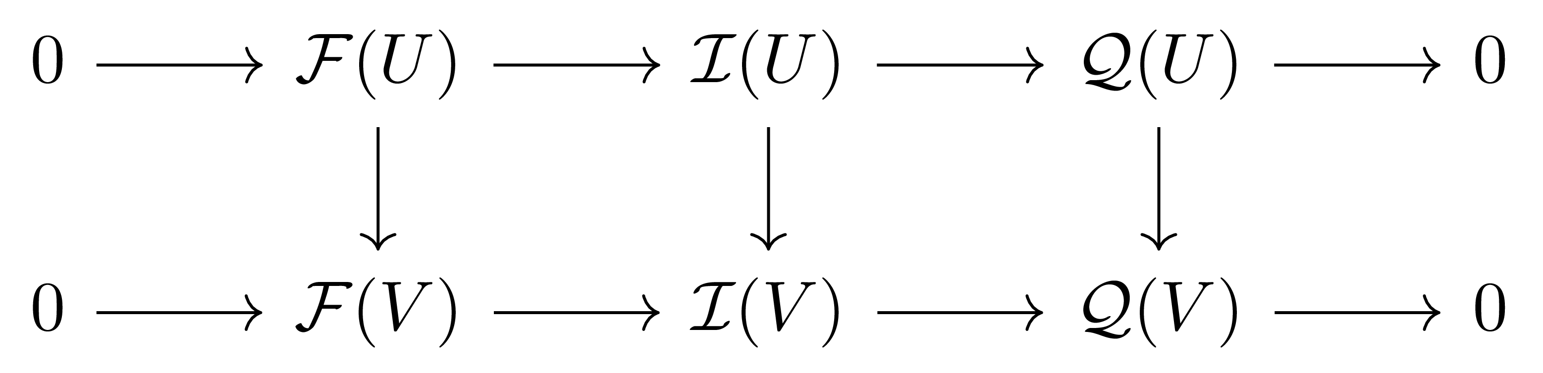
에서 diagram chase를 하면 된다. 여기서 \(\mathcal{F}\)는 가정에 의해 flasque이며 \(\mathcal{I}\)는 injective이므로 flasque이다. 이제 임의의 \(s\in \mathcal{Q}(V)\)에 대하여, \(\mathcal{I}(V)\rightarrow \mathcal{Q}(V)\)가 surjective이므로 \(s\)를 \(t\in \mathcal{I}(V)\)로 lift할 수 있으며, 다시 \(\mathcal{I}\)가 flasque임을 이용하여 \(t\)를 \(\overline{t}\in\mathcal{I}(U)\)로 올린 후 이를 \(\mathcal{Q}\)로 옮겨주어 \(\overline{s}\in \mathcal{Q}(U)\)를 정의하면 된다. 이제 \(\mathcal{Q}(U)\)에서의 원소 \(\overline{s}\vert_V-s\)는 \(\mathcal{F}(V)\)의 원소이고, 다시 \(\mathcal{F}\)의 flasqueness로부터 적당한 \(h\in \mathcal{F}(U)\)가 존재하여 \(h\vert_V=\overline{s}\vert_V-s\)이다. 이제 이로부터 \(\overline{s}-h\)는 정확히 \(s\in \mathcal{Q}(V)\)로 restrict하며 이로부터 \(\mathcal{Q}\)의 flasqueness를 얻는다.
이제 \(\Gamma(X, -)\)를 적용하여 long exact sequence
\[0 \to \Gamma(X, \mathcal{F}) \to \Gamma(X, \mathcal{I}) \to \Gamma(X, \mathcal{Q}) \xrightarrow{\delta} H^1(X, \mathcal{F}) \to H^1(X, \mathcal{I}) = 0\]을 얻자. 여기서 \(\mathcal{I}\)가 injective이므로 \(H^1(X, \mathcal{I}) = 0\)이다. 따라서
\[H^1(X, \mathcal{F}) \cong \coker(\Gamma(X, \mathcal{I}) \to \Gamma(X, \mathcal{Q}))\]이며, 이것이 \(0\)이 된다는 것을 보이기 위해 우리는 \(\Gamma(X, \mathcal{I})\rightarrow \Gamma(X, \mathcal{Q})\)가 surjective임을 보여야 한다. 이를 위해 임의의 \(s\in \Gamma(X, \mathcal{Q})\)가 주어졌다 하자. 그럼 임의의 \(x\in X\)에 대하여, stalk 레벨에서는 \(\mathcal{I}\rightarrow \mathcal{Q}\)가 surjective하므로 각각의 \(x\in X\)마다 적당한 \(t_x\in \mathcal{I}_x\)가 존재하여 \(t_x\)가 \(s_x\in \mathcal{Q}_x\)로 가도록 할 수 있다. 이제 \(t_x\)의 한 representative를 택하여, \(t_x\)가 \(\mathcal{I}(U_x)\)의 원소 인 것으로 생각하면 \(\mathcal{I}\)가 flasque이므로 이들 각각을 \(X\)에서의 global section \(T_x\)들로 확장할 수 있으며, 그럼 \(T_x\mid_{U_x}=s\mid_{U_x}\)이다.
이제 \(T_x\)들의 \(\Gamma(X,\mathcal{Q})\)에서의 image를 \(S_x\)라 하자. 그럼 \(S_x-S_y\)는 \(U_x\cap U_y\)에서 identically zero이며, 따라서 이를 \(U_x\cap U_y\) 위에서 \(\mathcal{F}\)의 section \(f_{xy}\)로 lift할 수 있다. 다시 \(\mathcal{F}\)의 flasqueness를 사용하면 이를 \(f_x\in \mathcal{F}(U_x)\)와 \(f_y\in \mathcal{F}(U_y)\) 각각으로 확장할 수 있고, 그럼 이 상황에서 \(T_x\)를 \(T'_x=T_x-f_x\)들로 대체하면 이것이 compatibility condition을 만족하고 따라서 이들을 붙인 것이 \(s\)의 preimage인 것을 안다.
마지막으로, long exact sequence에 의하여
\[H^i(X, \mathcal{F})\cong H^{i-1}(X, \mathcal{Q})\]이고, \(\mathcal{Q}\)가 flasque이므로 귀납법에 의하여 원하는 결과를 얻는다.
특히, 명제 16에 의하여 Godement resolution의 각 항 \(\mathcal{G}^p(\mathcal{F})\)는 flasque이므로 \(\Gamma(X, -)\)-acyclic이다. 즉, 모든 \(i > 0\)에 대해 \(H^i(X, \mathcal{G}^p(\mathcal{F})) = 0\)이다. 이제 결론을 내기 위해 우리가 필요한 것은 다음 결과이다.
명제 17 (Acyclic Resolution) \(\Gamma(X, -)\)-acyclic resolution \(0 \to \mathcal{F} \to \mathcal{A}^0 \to \mathcal{A}^1 \to \cdots\)이 주어지면
\[H^q(\Gamma(X, \mathcal{A}^\bullet)) \cong H^q(X, \mathcal{F})\]이 모든 \(q \geq 0\)에 대해 성립한다.
증명
\(\mathcal{F}\)의 injective resolution \(0 \to \mathcal{F} \to \mathcal{I}^\bullet\)을 고정하자. Comparison theorem ([호몰로지 대수학] §분해, ⁋정리 6)에 의해 acyclic resolution과 injective resolution 사이에 chain map \(f\colon \mathcal{A}^\bullet \to \mathcal{I}^\bullet\)이 존재한다. \(f\)의 mapping cone \(C(f)^\bullet\)을 생각하자. 각 차수에서
\[C(f)^n = \mathcal{A}^{n+1} \oplus \mathcal{I}^n\]이며, \(\mathcal{I}^n\)는 injective이므로 보조정리 9에 의해 flasque, 특히 \(\Gamma(X, -)\)-acyclic이다. 따라서 canonical short exact sequence
\[0 \to \mathcal{I}^n \to C(f)^n \to \mathcal{A}^{n+1} \to 0\]를 생각하면 양 끝 항이 \(\Gamma(X, -)\)-acyclic이므로 long exact sequence로부터 \(C(f)^n\) 역시 \(\Gamma(X, -)\)-acyclic임을 알 수 있다.
한편 \(f\)는 quasi-isomorphism이므로 \(C(f)^\bullet\)은 exact complex이다. ([호몰로지 대수학] §긴 완전열, ⁋따름정리 9) 뿐만 아니라 \(C(f)^\bullet\)은 위에서 살펴봤듯 \(\Gamma(X,-)\)-acyclic이므로, 여기에 \(\Gamma(X,-)\)를 취해 exact complex \(\Gamma(X, C(f)^\bullet)\)을 얻을 수 있으며 다시 [호몰로지 대수학] §긴 완전열, ⁋따름정리 9을 적용하여 이것을 chain map
\[\Gamma(X, f)\colon \Gamma(X, \mathcal{A}^\bullet) \to \Gamma(X, \mathcal{I}^\bullet)\]이 quasi-isomorphism이라는 조건으로 바꿔줄 수 있다. 이로부터
\[H^q(\Gamma(X, \mathcal{A}^\bullet)) \cong H^q(\Gamma(X, \mathcal{I}^\bullet)) = H^q(X, \mathcal{F})\]을 얻는다.
명제 17는 명제 16과 함께 Godement resolution이 실제로 sheaf cohomology를 계산하기에 충분하다는 것을 보장한다. 즉, flasque resolution \(\mathcal{G}^\bullet(\mathcal{F})\)의 global section을 취하여 얻은 complex \(\Gamma(X, \mathcal{G}^\bullet(\mathcal{F}))\)의 cohomology가 \(H^\bullet(X, \mathcal{F})\)와 일치한다.
Spectral Sequence
Sheaf cohomology의 가장 강력한 응용 중 하나는 spectral sequence를 통한 cohomology의 계산이다. 우리는 이번 섹션에서 구체적인 계산으로 이 글을 마무리하기로 한다. 지금 소개하는 명제들은 일반적인 위상수학적 설정에서 성립하지만, 우리는 주로 variety와 quasi-coherent sheaf에의 적용을 염두에 둘 것이므로 이 카테고리에 담았다.
연속함수 \(f : X \to Y\)와 sheaf \(\mathcal{F}\)를 고정하자. 그럼 [위상수학] §층, ⁋보조정리 11와 [범주론] §수반함자, ⁋정리 9로부터 direct image functor \(f_\ast: \Sh(X)\rightarrow \Sh(Y)\)는 left exact functor임을 안다. 따라서 우리는 [호몰로지 대수학] §Derived Functor에서와 마찬가지로 \(f_\ast\)의 right derived functor를
\[R^q f_\ast \mathcal{F} := H^q(f_\ast \mathcal{I}^\bullet)\]로 정의할 수 있다. 여기서 \(\mathcal{I}^\bullet\)은 \(\mathcal{F}\)의 injective resolution이다. 정의에 의해 \(q=0\)일 때 \(R^0 f_\ast \mathcal{F}=f_\ast \mathcal{F}\)이며 \(\mathcal{F}\)가 injective이면 \(\mathcal{F}\) 자체로 injective resolution을 이루므로 \(R^qf_\ast \mathcal{F}=0\)이 성립한다.
이제 \(\mathcal{F}\)의 Godement resolution \(\mathcal{G}^\bullet(\mathcal{F})\)을 생각하자. 직관적으로 우리가 하고 싶은 것은 \(\mathcal{G}^p(\mathcal{F})\) 각각에 대한 injective resolution을 잡은 후, Godement resolution의 differential \(\mathcal{G}^p(\mathcal{F})\rightarrow \mathcal{G}^{p+1}(\mathcal{F})\)을 [호몰로지 대수학] §분해, ⁋정리 6을 통해 horizontal differential을 정의해주는 것이다.
정의 18 (Cartan-Eilenberg Resolution) Abelian category에서 cochain complex \(K^\bullet\)의 Cartan-Eilenberg resolution카르탕-아일렌베르크 분해은 double complex \(I^{p,q}\)와 augmentation \(K^\bullet \to I^{\bullet,0}\)으로 이루어진 데이터로, 다음 조건들을 만족하는 것이다.
- 각 열 \(I^{p,\bullet}\)은 \(K^p\)의 injective resolution이다.
-
각 행의 cohomology \(H^p(I^{\bullet,q})\)는 \(H^p(K^\bullet)\)의 injective resolution을 이룬다. 즉, chain complex
\[\cdots \to H^p(I^{\bullet,q-1}) \to H^p(I^{\bullet,q}) \to H^p(I^{\bullet,q+1}) \to \cdots\]은 \(H^p(K^\bullet)\)의 injective resolution이다.
이 정의의 핵심은 위에서 언급한 직관만으로는 Cartan-Eilenberg resolution이 얻어지지 않는다는 것으로, 특히 각 행의 cohomology가 \(H^p(K^\bullet)\)의 horizontal resolution을 이룬다는 것이 존재성의 증명에 핵심적인 요소이다. 우리는 Cartan-Eilenberg resolution의 존재성은 별도로 증명하지 않지만, 기본적으로는 [호몰로지 대수학] §분해, ⁋보조정리 7를 반복적으로 적용하여 얻을 수 있다.
이제 complex \(f_\ast\mathcal{G}^\bullet(\mathcal{F})\)의 Cartan-Eilenberg resolution \(\mathcal{I}^{p,q}\)을 고정하자. 그럼 정의에 의해 각 열 \(\mathcal{I}^{p,\bullet}\)은 \(f_\ast\mathcal{G}^p(\mathcal{F})\)의 injective resolution이며, 각 행의 horizontal cohomology \(H^p(\mathcal{I}^{\bullet,q})\)는 \(H^p(f_\ast\mathcal{G}^\bullet(\mathcal{F})) = R^p f_\ast\mathcal{F}\)의 injective resolution을 이룬다.
우리는 이 spectral sequence가 1사분면에 있으므로, total complex \(\Tot(\mathcal{I})^\bullet\)의 cohomology로 수렴한다는 것을 안다. 구체적인 계산을 위해 Godement 방향의 \(p\)로 filtration을 걸자. 그럼 우리는 우선 \(E_1\) page를
\[\mathcal{H}^{p,q} := H^p(\mathcal{I}^{\bullet, q})\]로 쓸 수 있다. 이 때 vertical differential은 injective resolution의 differential이 cohomology level로 내려와서 유도하는 사상 \(\mathcal{H}^{p,q}\rightarrow \mathcal{H}^{p,q+1}\)이며, \(E_2\) page는 이 vertical complex의 cohomology sheaf
\[E_2^{p,q} = H^q(\mathcal{H}^{p,\bullet})\]이다. 한편 \(\mathcal{I}^{\bullet,\bullet}\)이 Cartan resolution이라는 것으로부터, 우리는 각각의 \(\mathcal{H}^{p,\bullet}\)이 \(R^p f_\ast \mathcal{F}\)의 injective resolution임을 안다. 우리는 이 spectral sequence를 Leray spectral sequence라 부른다.
한편 \(q\)방향의 filtration으로부터 오는 spectral sequence를 생각하면, 그 \(E_1\) page는
\[E_1^{p,q} = H^q(\mathcal{I}^{p,\bullet})\]로 주어진다. 이 때, 각 \(p\)에 대하여 \(\mathcal{I}^{p,\bullet}\)은 \(f_\ast \mathcal{G}^p(\mathcal{F})\)의 injective resolution이므로, injective resolution의 exactness에 의하여
\[E_1^{p,q} = \begin{cases} f_\ast \mathcal{G}^p(\mathcal{F}) & \text{if $q = 0$} \\ 0 & \text{if $q > 0$} \end{cases}\]이며 \(d_1\)-differential은 \(E_1^{p,0} = f_\ast \mathcal{G}^p(\mathcal{F})\)에서 \(E_1^{p+1,0} = f_\ast \mathcal{G}^{p+1}(\mathcal{F})\)로 가는 사상으로, Godement resolution의 differential \(f_\ast \mathcal{G}^p(\mathcal{F}) \to f_\ast \mathcal{G}^{p+1}(\mathcal{F})\)에 해당한다. 즉, \(E_2\) page는 complex
\[0 \to f_\ast \mathcal{F} \to f_\ast \mathcal{G}^0(\mathcal{F}) \to f_\ast \mathcal{G}^1(\mathcal{F}) \to \cdots\]의 cohomology sheaf이고, 이것은 \(R^q f_\ast\)의 정의에 의해
\[E_2^{p,q} = \begin{cases} R^p f_\ast \mathcal{F} & \text{if $q = 0$} \\ 0 & \text{if $q > 0$} \end{cases}\]으로 주어진다. 따라서 \(\mathcal{I}^{\bullet,\bullet}\)의 total complex의 cohomology가 \(R^n f_\ast \mathcal{F}\)으로 수렴해야 하는 것을 안다.
이제 이 결과에 global section functor \(\Gamma(Y,-)\)을 취하여 위의 논의를 다시 살펴보자. 즉 우리는 double complex
\[\mathcal{J}^{p,q}=\Gamma(Y, \mathcal{I}^{p,q})\]와 그 total complex \(\Tot(\mathcal{J})^\bullet\)을 생각한다. 그럼 위와 마찬가지 계산으로, \(p\)방향의 filtration은 \(E_1\) page에서
\[E_1^{p,q}=H^p(\mathcal{J}^{\bullet, q})=\Gamma(Y, \mathcal{H}^{p,q})\]이며, \(\mathcal{H}^{p,q}\)는 \(R^pf_\ast \mathcal{F}\)의 injective resolution이므로 그 cohomology가 \(H^q(Y, R^p f_\ast \mathcal{F})\)으로 나오는 것을 안다.
한편, \(q\) 방향 filtration의 경우 \(E_1\) page는
\[E_1^{p,q}=H^q(\Gamma(Y, \mathcal{I}^{p,\bullet}))\]이며, 이 때 각각의 \(\mathcal{I}^{p,\bullet}\)은 Cartan-Eilenberg resolution의 정의에 의하여 injective resolution이므로 flasque이고 (보조정리 9), flasque sheaf는 \(\Gamma\)-acyclic이므로 \(q>0\)에서의 항들이 소멸하며 남는 것은
\[E_1^{p,0}=\Gamma(Y, f_\ast \mathcal{G}^p (\mathcal{F}))=\Gamma(X, \mathcal{G}^p(\mathcal{F}))\]이며 여기서의 differential은 Godement differential이다. 따라서 \(E_2\) page는
\[E_2^{n,0}=H^n(\Gamma(X, \mathcal{G}^\bullet(\mathcal{F}))=H^n(X, \mathcal{F})\]가 되며, 따라서 다음을 얻는다.
명제 19 (Leray Spectral Sequence) 연속함수 \(f : X \to Y\)와 sheaf \(\mathcal{F}\)에 대하여, 다음의 \(E_2\) page를 가지는 spectral sequence가 존재한다.
\[E_2^{p,q} = H^p(Y, R^q f_* \mathcal{F}) \Rightarrow H^{p+q}(X, \mathcal{F}).\]기하학적으로 이는 \(f:X\rightarrow Y\)가 fibration일 때 그 의미가 가장 명확한데, 이 경우 이 spectral sequence가 뜻하는 바는 \(X\) 위의 cohomology를 계산하기 위해서는 \(Y\) 위에서의 cohomology를 먼저 계산한 후, 각 점의 fiber 위에서의 cohomology를 higher sheaf \(R^q f_* \mathcal{F}\)로 기억한 뒤, 이들을 \(Y\) 위에서 합성하면 된다는 것이다.
이제 Leray spectral sequence의 가장 낮은 차원에서는 다음의 exact sequence를 얻을 수 있다.
따름정리 20 (Five-Term Exact Sequence) 연속함수 \(f : X \to Y\)와 sheaf \(\mathcal{F}\)에 대하여, Leray spectral sequence로부터 다음의 exact sequence
\[0 \to H^1(Y, f_* \mathcal{F}) \to H^1(X, \mathcal{F}) \to H^0(Y, R^1 f_* \mathcal{F}) \overset{d_2}{\to} H^2(Y, f_* \mathcal{F}) \to H^2(X, \mathcal{F})\]를 얻는다.
증명
Leray spectral sequence \(E_2^{p,q} = H^p(Y, R^q f_* \mathcal{F}) \Rightarrow H^{p+q}(X, \mathcal{F})\)의 \(E_2\) page에서 \(p+q \leq 2\)인 항목들을 고려하자. [호몰로지 대수학] §스펙트럼 열, ⁋정의 5에 의해 우리는
\[E_\infty^{p,q} \cong \gr^p H^{p+q} = F^p H^{p+q}/F^{p+1}H^{p+q}\]임을 안다. 특히, 이는 first quadrant spectral sequence이므로 충분히 큰 \(r\)에서 \(E_r^{p,q} = E_\infty^{p,q}\)이다. ([호몰로지 대수학] §스펙트럼 열, ⁋명제 6)
우선 \(p+q = 1\)인 성분들을 보면, 오직 두 개의 항 \(E_2^{1,0}\)와 \(E_2^{0,1}\)만이 존재한다. 그런데 차수를 고려하면 \(E_2^{1,0}\)로 들어오거나 나가는 differential은 모두 0이므로 \(E_2^{1,0} = E_\infty^{1,0}\)이다. 반면, \(E_2^{0,1}\)에서 \(E_2^{2,0}\)으로 가는 \(d_2\)가 비자명할 수 있으므로 \(E_\infty^{0,1} = \ker(d_2: E_2^{0,1} \to E_2^{2,0})\)이다. 그럼 filtration에 의하여
\[0 \to E_\infty^{1,0} \to H^1(X, \mathcal{F}) \to E_\infty^{0,1} \to 0\]이 exact하며, 여기서 \(E_\infty^{1,0} = E_2^{1,0}\)이고 \(E_\infty^{0,1} = \ker(d_2) \hookrightarrow E_2^{0,1}\)이므로 이를 합치면 다음의 exact sequence
\[0 \to E_2^{1,0} \to H^1(X, \mathcal{F}) \to E_2^{0,1} \xrightarrow{d_2} E_2^{2,0}\]를 얻는다.
이제 증명을 완성하기 위해 \(p+q = 2\)인 성분 \(E_2^{2,0}\), \(E_2^{1,1}\), \(E_2^{0,2}\)을 보자. 마찬가지 이유로 \(d_2 : E_2^{0,1} \to E_2^{2,0}\)가 유일한 비자명한 differential이며, 이 differential이 정의하는 \(E_3\) page에서
\[E_3^{0,2} = \ker(d_2 : E_2^{0,2} \to E_2^{2,1}), \qquad E_3^{2,0} = \operatorname{coker}(d_2 : E_2^{0,1} \to E_2^{2,0})\]이고, 다시 차수를 분석하면 \(E_3^{p,q} = E_\infty^{p,q}\)이므로
\[E_\infty^{2,0} = E_3^{2,0} = \operatorname{coker}(d_2 : E_2^{0,1} \to E_2^{2,0})\]이다. 우리는 지금까지 exact sequence
\[0 \to E_2^{1,0} \to H^1(X, \mathcal{F}) \to E_2^{0,1} \xrightarrow{d_2} E_2^{2,0}\]가 존재함을 보였으며, 위의 계산에서
\[E_\infty^{2,0} = E_3^{2,0} = \operatorname{coker}(d_2: E_2^{0,1} \to E_2^{2,0})\]이므로 filtration을 통해 \(F^2 H^2 \hookrightarrow H^2(X, \mathcal{F})\)로 넣어주면
\[E_2^{0,1} \overset{d_2}{\to} E_2^{2,0} \to H^2(X, \mathcal{F})\]이 exact하다. 이를 합치면 원하는 결과를 얻는다.
이 exact sequence는 \(d_2\)-differential의 존재가 cohomology의 계산에 어떤 제약을 주는지를 보여주며, \(H^i(X, \mathcal{F}) \cong H^i(Y, f_* \mathcal{F})\)라는 직관을 좋은 경우에서는 정당화해준다.
마지막으로 우리는 Čech cohomology와 derived functor cohomology의 관계를 spectral sequence로 기술할 수 있다.
명제 21 (Čech-to-Derived Functor Spectral Sequence) 위상공간 \(X\) 위의 sheaf \(\mathcal{F}\)와 open cover \(\mathcal{U}\)에 대하여, spectral sequence
\[E_2^{p,q} = \check{H}^p(\mathcal{U}, \mathcal{H}^q(\mathcal{F})) \Rightarrow H^{p+q}(X, \mathcal{F})\]이 존재한다. 여기서 \(\mathcal{H}^q(\mathcal{F})\)는 presheaf \(U \mapsto H^q(U, \mathcal{F})\)의 sheafification이다.
증명
\(\mathcal{F}\)의 Godement resolution \(\mathcal{G}^\bullet(\mathcal{F})\)을 잡고, double complex \(C^{p,q} = \check{C}^p(\mathcal{U}, \mathcal{G}^q(\mathcal{F}))\)를 구성한다. 두 filtration으로부터 얻어지는 두 spectral sequence가 같은 total cohomology \(H^{p+q}(X, \mathcal{F})\)에 수렴한다는 것은 [호몰로지 대수학] §스펙트럼 열, ⁋예시 11에 의한 것이며, 이 때 Godement sheaf \(\mathcal{G}^q(\mathcal{F})\)가 flasque이므로 보조정리 10에 의해 Čech-acyclic이 되어 위에서의 계산과 같은 vanishing을 사용하면 된다.
이 spectral sequence는 정리 11를 더 넓은 맥락에서 이해할 수 있게 해준다. 만일 \(\mathcal{U}\)의 모든 유한한 교집합에서 \(\mathcal{F}\)가 acyclic이면, \(\mathcal{H}^q(\mathcal{F}) = 0\)이 모든 \(q > 0\)에 대해 성립하므로, \(E_2\) page에서 \(q > 0\)인 항목이 모두 소멸하여 \(E_2^{p,0} = \check{H}^p(\mathcal{U}, \mathcal{F}) \cong H^p(X, \mathcal{F})\)를 얻는다. 즉, Čech-to-derived functor spectral sequence는 정리 11를 포함하는 더 일반적인 결과라 할 수 있다.
Line Bundle의 Classification
앞서 우리는 line bundle이 transition function \(g_{ij} \in \mathcal{O}_X^\ast(U_i \cap U_j)\)들로 결정된다는 것을 보았다 (§선다발과 벡터다발, ⁋명제 2). Transition function들은 cocycle condition \(g_{ij}g_{jk} = g_{ik}\)을 만족하는데, 이는 multiplicative notation으로 쓴 Čech 1-cocycle condition에 정확히 해당한다. 또한 line bundle의 isomorphism은 각 \(U_i\) 위에서의 함수 \(h_i \in \mathcal{O}_X^\ast(U_i)\)에 의해 \(g_{ij} \mapsto h_i g_{ij} h_j^{-1}\)로 transition function이 변하는 것이므로, 이 역시 Čech 1-coboundary에 의한 동치관계와 일치한다. 즉, line bundle의 isomorphism class는 \(\check{H}^1(X, \mathcal{O}_X^\ast)\)의 원소와 자연스럽게 대응된다.
이 관찰을 엄밀하게 정리하면 다음을 얻는다. 여기서 주의할 점은 \(\mathcal{O}_X^\ast\)가 곱셈적 구조를 갖는 sheaf of (abelian) groups이므로, Čech cohomology에서 coboundary 관계가 덧셈적이 아닌 곱셈적으로 표현된다는 것이다. 구체적으로 1-coboundary는 \((g_{ij}) = (h_i \cdot h_j^{-1})\)의 꼴이다.
명제 22 \(\check{H}^1(X, \mathcal{O}_X^\ast) \cong \Pic(X)\)이다.
증명
우선 \(\check{H}^1(X, \mathcal{O}_X^\ast)\)에서 \(\Pic(X)\)로의 map을 정의한다. Čech 1-cocycle \((g_{ij}) \in \check{Z}^1(\mathcal{U}, \mathcal{O}_X^\ast)\)가 주어졌다 하고, 이를 transition function으로 하는 line bundle \(\mathcal{L}\)을 만들자. 이를 위해 우리는 각 \(U_i\) 위에서는 trivial bundle \(U_i \times \mathbb{A}^1\)을 잡고, \(U_i \cap U_j\) 위에서는 \((p, t) \mapsto (p, g_{ij}(p)t)\)으로 붙여준다. 이 때, cocycle condition \(g_{ij}g_{jk} = g_{ik}\)에 의해 이 gluing이 consistent하므로 well-defined line bundle이 얻어진다.
한편, coboundary에 의해 동치인 두 cocycle \(g_{ij}^{\mathcal{L}} = h_i g_{ij}^{\mathcal{M}} h_j^{-1}\)이 주어지면, 이에 대응하는 두 line bundle 사이의 isomorphism을 \(\varphi_i: \mathcal{L}\vert_{U_i} \to \mathcal{M}\vert_{U_i}\), \(v \mapsto h_i^{-1} v\)로 정의할 수 있다. 그러면 \(\varphi_i\)와 \(\varphi_j\)가 \(U_i \cap U_j\)에서 compatible임은
\[g_{ij}^{\mathcal{M}} \cdot \varphi_j(v) = g_{ij}^{\mathcal{M}} h_j^{-1} v = h_i^{-1} (h_i g_{ij}^{\mathcal{M}} h_j^{-1}) v = h_i^{-1} g_{ij}^{\mathcal{L}} v = \varphi_i(g_{ij}^{\mathcal{L}} v)\]에서 확인할 수 있으며, 따라서 map \(\check{H}^1(\mathcal{U}, \mathcal{O}_X^\ast) \to \Pic(X)\)가 well-defined이다.
역으로, 임의의 line bundle \(\mathcal{L}\)은 (§선다발과 벡터다발, ⁋정의 1)에 의해 적당한 open cover \(\mathcal{U}\) 위에서 transition function \(g_{ij}\)로 표현되며, 이는 Čech 1-cocycle을 이룬다. Line bundle isomorphism은 정확히 coboundary에 의한 동치관계에 해당하므로, 이 map의 kernel은 coboundary들이다. 따라서 \(\check{H}^1(\mathcal{U}, \mathcal{O}_X^\ast) \to \Pic(X)\)는 injective이다. 이제 direct limit을 취하면 \(\check{H}^1(X, \mathcal{O}_X^\ast) \cong \Pic(X)\)를 얻는다.
이 명제는 line bundle의 classification이 cohomology의 계산으로 귀결된다는 것을 보여준다. 즉, \(\Pic(X)\)의 원소를 분류하는 문제는 이제 \(\mathcal{O}_X^\ast\)-valued Čech 1-cocycle을 분류하는 문제가 되며, 이는 어쨌든 명시적인 계산이 가능하다는 점에서 고무적이다. 다음 글 §사영공간의 코호몰로지에서 우리는 \(\mathbb{P}^n\) 위의 line bundle \(\mathcal{O}(d)\)의 cohomology를 계산한다.
참고문헌
[Har] R. Hartshorne, Algebraic geometry, Graduate Texts in Mathematics, Springer, 1977. [Sha] I. R. Shafarevich, Basic Algebraic Geometry I: Varieties in Projective Space, Springer, 2013. [God] R. Godement, Topologie algébrique et théorie des faisceaux, Hermann, 1958. [Wei] C. A. Weibel, An Introduction to Homological Algebra, Cambridge Studies in Advanced Mathematics 38, Cambridge University Press, 1994.
-
더 일반적으로, [[위상수학] §층, §층들의 가환범주에서 살펴보았듯 임의의 위상공간 \(X\) 위에 정의된 sheaf들의 category \(\Sh(X)\)는 abelian category를 이룬다. ↩
댓글남기기