
카테고리 \(\Ch(\mathcal{A})\)
[범주론] §아벨 카테고리에서 우리는 chain complex들의 카테고리 \(\Ch(\mathcal{A})\)가 존재하며, abelian category가 된다는 것을 언급하였는데, 이번 절에서 우리는 조금 더 구체적으로 이 주장을 살펴본다. 우선 \(\Ch(\mathcal{A})\)에서의 morphism은 다음과 같이 주어진다.
정의 1 두 chain complex \(C_\bullet, D_\bullet\)에 대하여, 이들 사이의 chain map사슬변환 \(f_\bullet:C_\bullet\rightarrow D_\bullet\)은 다음의 diagram
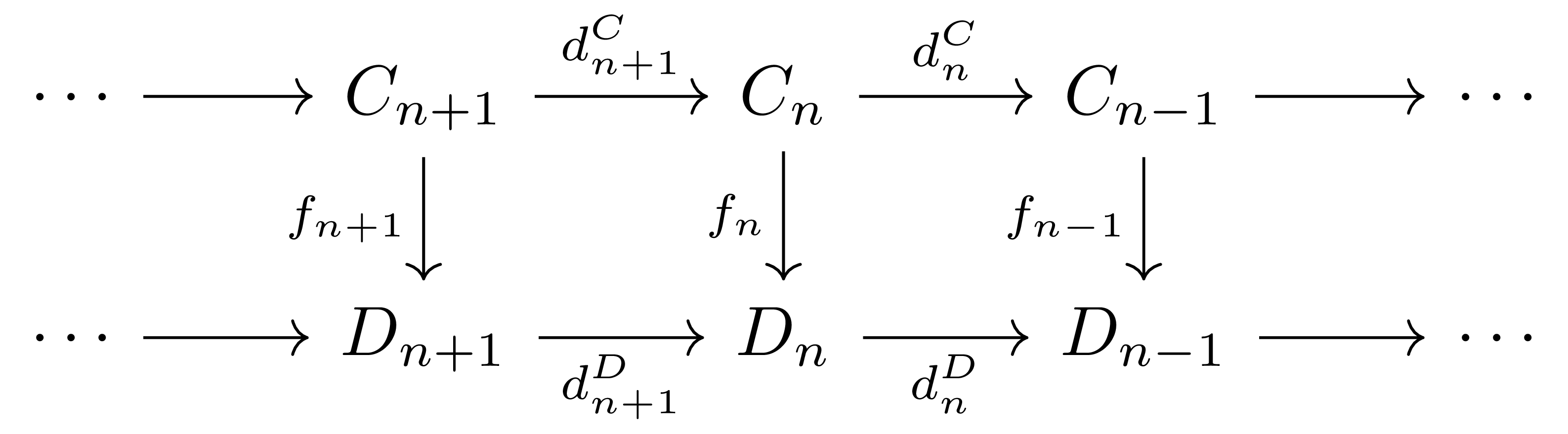
을 commute하도록 하는 \(f_n:C_n\rightarrow D_n\)들의 모임이다.
즉, \(f_\bullet\)이 chain map이라는 것은 모든 \(n\)에 대하여
\[f_{n-1}\circ d_n^C=d_n^D\circ f_n\]이 성립하는 것이다. 혼동의 여지가 없을 때에는 \(d^C\)와 \(d^D\)를 모두 \(d\)로만 적는다. 그럼 category \(\Ch(\mathcal{A})\)를
- \(\mathcal{A}\)의 chain complex들의 모임 \(\obj(\Ch(\mathcal{A}))\),
- Chain complex \(C_\bullet\)에서 \(D_\bullet\)으로의 chain map들의 모임 \(\Mor_{\Ch(\mathcal{A})}(C_\bullet,D_\bullet)\)
으로 정의하면 \(\Ch(\mathcal{A})\)가 category가 된다는 것이 자명하다. 이 때, \(\id_{C_\bullet}\)은 모든 \(n\)에 대하여 \(\id_n:C_n\rightarrow C_n\)이 \(\id_{C_n}\)으로 정의된 \(\id_\bullet:C_\bullet\rightarrow C_\bullet\)이며, chain map들의 합성은
\[g_\bullet\circ f_\bullet=(g_n\circ f_n)_{n\in\mathbb{Z}}\]으로 주어진다.
뿐만 아니라, category \(\Ch(\mathcal{A})\)는 \(\Ab\)-category이다. 두 chain map \(f_\bullet,g_\bullet:C_\bullet\rightarrow D_\bullet\)이 주어졌다면 이들의 합을
\[f_\bullet+g_\bullet=(f_n+g_n)_{n\in\mathbb{Z}}\]으로 정의하면 \(\Mor_{\Ch(\mathcal{A})}(C_\bullet,D_\bullet)\)이 abelian group이 되고, 또 두 chain complex \(C_\bullet,D_\bullet\)이 주어진다면 이들의 곱 \(C_\bullet\oplus D_\bullet\)은1 다음의 chain complex
\[C_\bullet\oplus D_\bullet:\quad \cdots \longrightarrow C_{n+1}\oplus D_{n+1}\overset{d_{n+1}^C\oplus d_{n+1}^D}{\longrightarrow}C_n\oplus D_n\overset{d_{n}^C\oplus d_{n}^D}{\longrightarrow}C_{n-1}\oplus D_{n-1}\longrightarrow\cdots\]으로 정의하면 되기 때문이다. Zero object는 다음의 chain complex
\[\cdots\rightarrow 0\rightarrow 0\rightarrow 0\rightarrow\cdots\]이다.
이제 \(\Ch(\mathcal{A})\)가 abelian category라는 것을 보이기 위해서는 임의의 chain map \(f_\bullet:C_\bullet \rightarrow D_\bullet\)의 kernel과 cokernel을 정의하면 충분하다. 우선 각각의 \(n\)에 대하여, \(f_n:C_n \rightarrow D_n\)은 abelian category \(\mathcal{A}\)에서의 morphism이므로 \(i_n:\ker f_n\rightarrow C_n\)과 \(p_n:D_n\rightarrow \coker f_n\)을 갖는다. 다음의 diagram
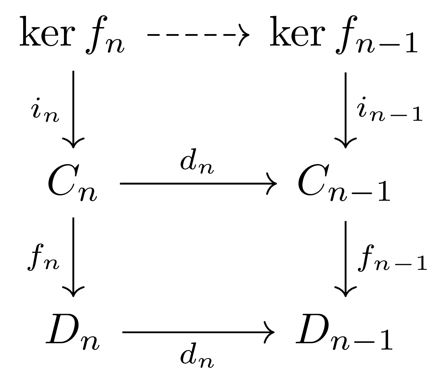
을 생각하자. 그럼
\[f_{n-1}\circ d_n\circ i_n=d_n\circ f_n\circ i_n=0\]이므로, \(\ker f_{n-1}\)의 universal property로부터 morphism \(\ker f_n\rightarrow \ker f_{n-1}\)이 자연스럽게 유도된다. 비슷하게 \(\coker f_n\rightarrow \coker f_{n-1}\) 또한 정의되며, 이 정보들은 각각 두 chain complex
\[\ker(f_\bullet):\qquad \cdots\longrightarrow \ker f_{n+1}\longrightarrow \ker f_n\longrightarrow \ker f_{n-1}\longrightarrow\cdots\]과
\[\coker(f_\bullet):\qquad \cdots\longrightarrow \coker f_{n+1}\longrightarrow \coker f_n\longrightarrow \coker f_{n-1}\longrightarrow\cdots\]을 각각 구성한다. 이렇게 정의한 \(\ker(f_\bullet)\)이 \(\Ch(\mathcal{A})\)에서 \(f_\bullet\)의 kernel이 된다는 것을 보이기 위해서는 다음의 universal property
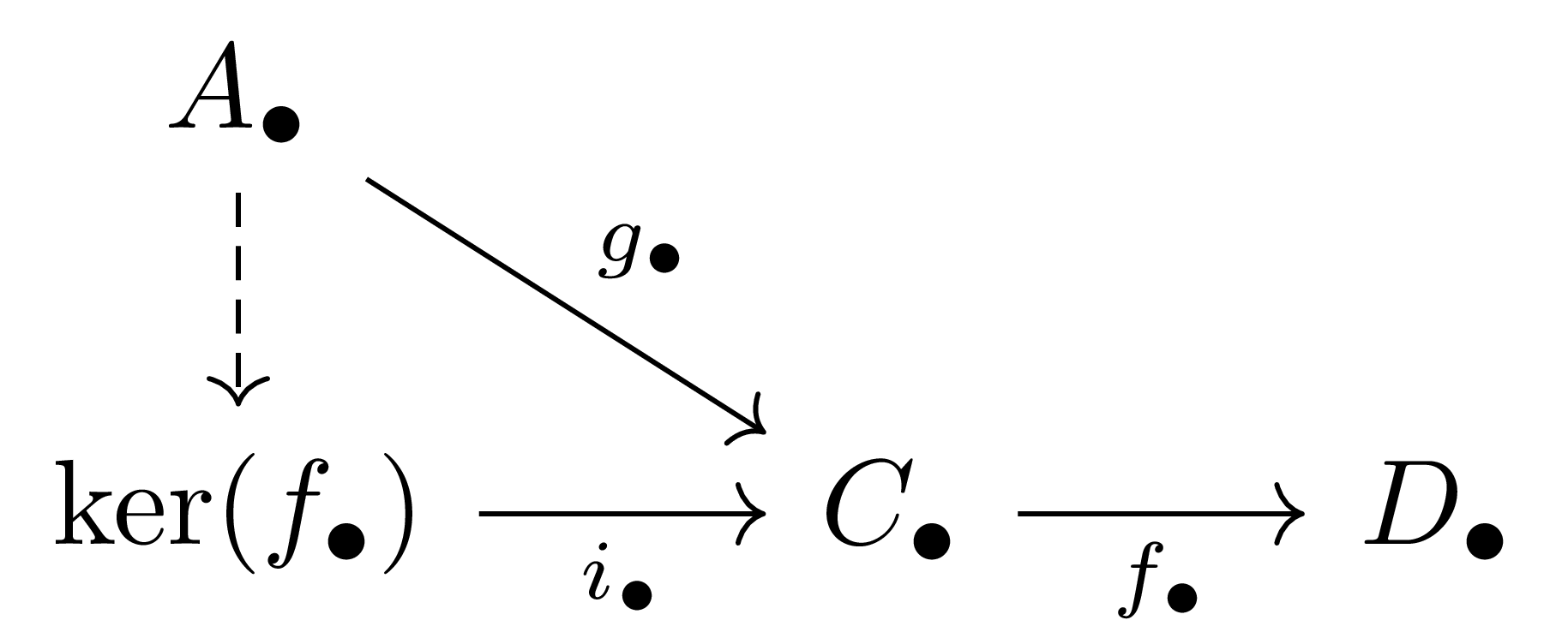
을 보여야 하는데, 다시 이를 위해서는 우선 각각의 \(n\)에 대하여 다음 diagram
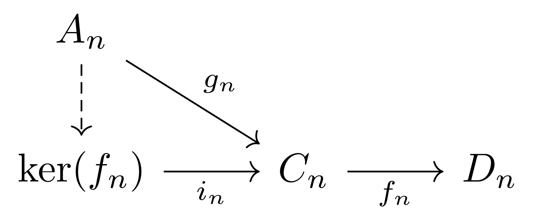
을 통해 \(j_n:A_n\rightarrow \ker f_n\)을 만든 후, \(j_\bullet\)이 chain map임을 보이면 충분하다. 즉, 다음 diagram
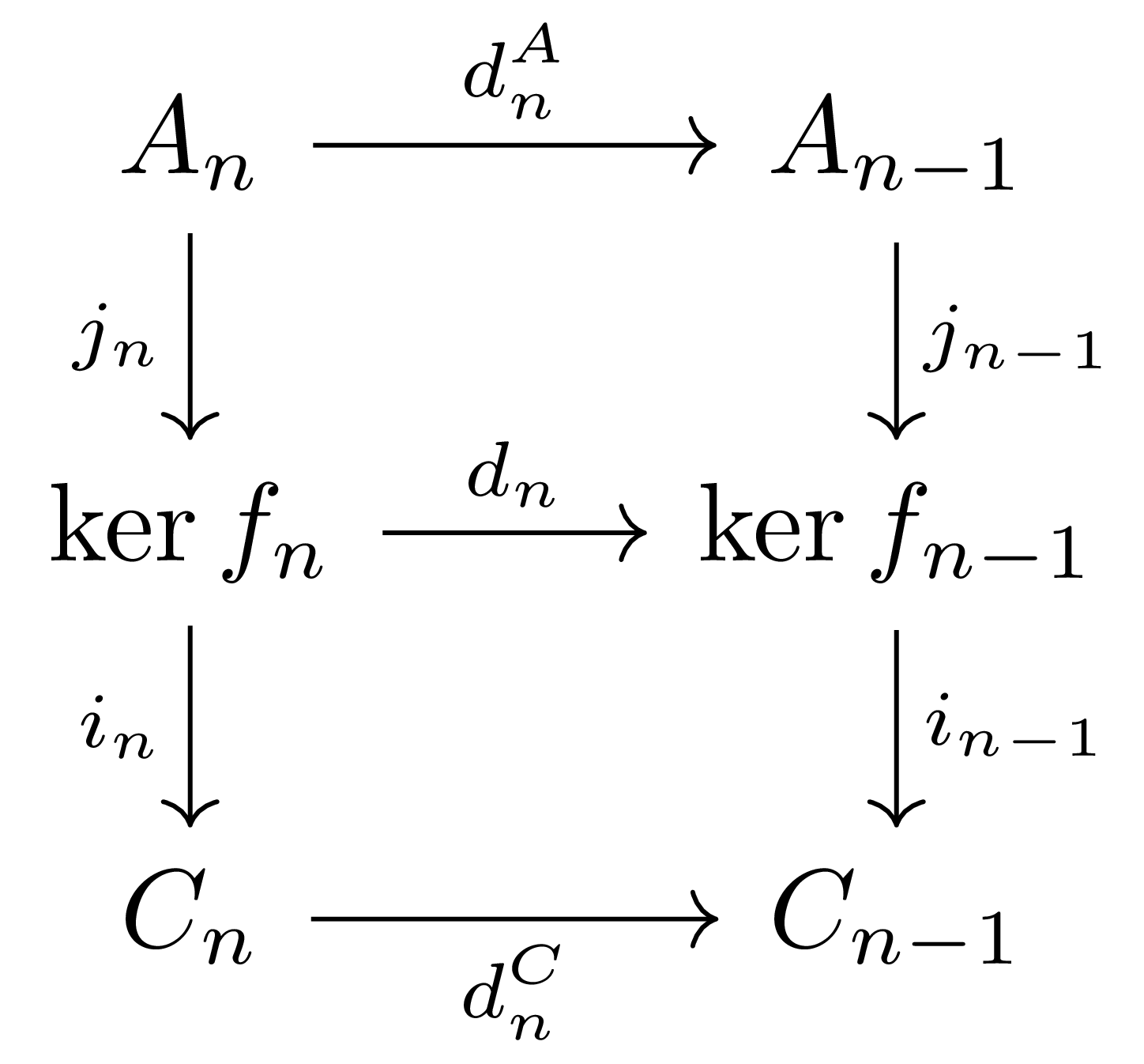
의 위쪽 사각형이 commute한다는 것을 증명하면 된다. 그런데 kernel은 항상 monomorphism이므로, 이를 위해서는
\[i_{n-1}\circ(j_{n-1}\circ d_n^A)=i_{n-1}\circ(d_n\circ j_n)\]이 성립한다는 것만 보이면 충분하고, 이는 정의에 의해 자명하므로 \(\ker(f_\bullet)\)은 실제로 \(f_\bullet\)의 kernel이 된다. 비슷하게 \(\coker(f_\bullet)\)이 \(\Ch(\mathcal{A})\)에서 \(f_\bullet\)의 cokernel이 된다는 것을 확인할 수 있다.
마지막으로 임의의 monomorphism \(f_\bullet\)이 \(\ker(\coker f_\bullet)\)와 같고, 임의의 epimorphism \(f_\bullet\)은 \(\coker(\ker f_\bullet)\)와 같다는 것을 보여야 한다. 이는 우선 \(f_\bullet\)이 monomorphism (resp. epimorphism)인 것과, 모든 \(n\)에 대하여 \(f_n\)이 monomorphism (resp. epimorphism)인 것이 동치임을 증명한 후, 각 차수별로 abelian category의 조건을 사용한 후 합쳐주면 된다. 이 과정은 위와 거의 동일하므로, 자세한 논증은 생략하기로 한다.
호몰로지
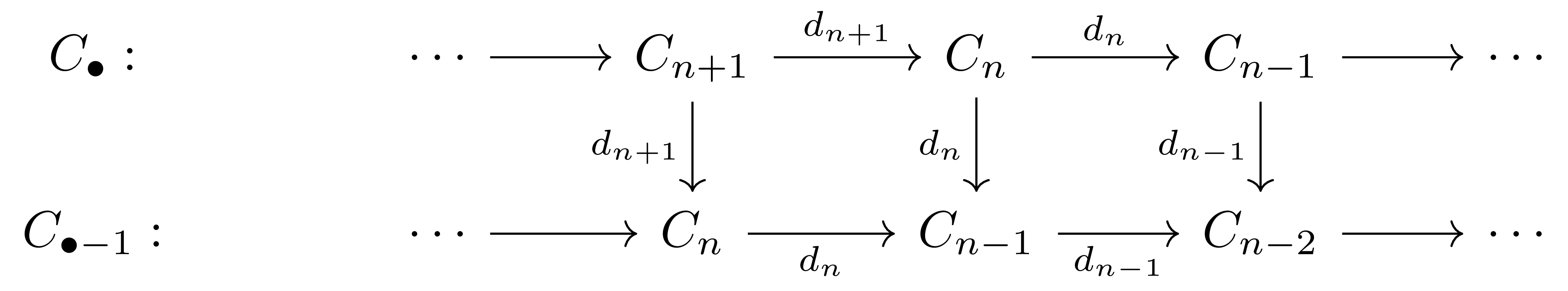
Chain complex \(C_\bullet\)을 고정하고, 새로운 chain complex \(C_{\bullet-1}\)을
\[C_{\bullet-1}:\qquad\cdots\longrightarrow\underbrace{C_n}_\text{\small degree $n+1$}\overset{d_n}{\longrightarrow}\underbrace{C_{n-1}}_\text{\small degree $n$}\overset{d_{n-1}}{\longrightarrow}\underbrace{C_{n-2}}_\text{\small degree $n-1$}\longrightarrow\cdots\tag{1}\]으로 정의하자. 즉 \(C_{\bullet-1}\)은 \(C_\bullet\)을 한 칸씩 옮겨서 얻어지는 chain complex이다. 이제 chain map \(d_\bullet:C_\bullet\rightarrow C_{\bullet-1}\)을 다음의 diagram
와 같이 정의하자. 그럼 \(\ker (d_\bullet)\)이 잘 정의되며, 다음의 diagram
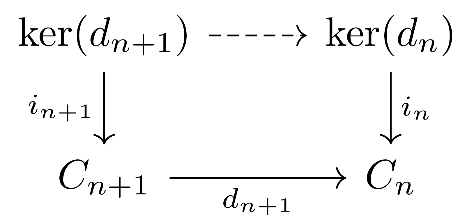
을 고려하면 \(d_{n+1}\circ i_{n+1}=0\)인 것과 \(i_n\)이 monomorphism인 것으로부터 \(\ker(d_\bullet)\)의 differential은 모두 zero map임을 알 수 있다.
마찬가지로 \(\coker(d_\bullet)\) 또한 잘 정의되며, 이들 사이의 differential 또한 0이 된다. 위에서 살펴본 \(\ker(d_\bullet)\)의 \(n\)번째 성분이 \(\ker d_n\rightarrow C_n\)인 것과는 달리, \(\coker(d_\bullet)\)의 \(n\)번째 성분은 \(C_{n-1}\rightarrow \coker(d_n)\)이므로 약간의 혼동이 있을 수 있으므로 우리는 다시 차수를 하나씩 옮겨서 chain complex \(\coker(d_{\bullet+1})\)를 생각한다.
이제
\[\im(d_{\bullet+1})=\ker(C_\bullet\rightarrow \coker(d_{\bullet+1}))\]으로 생각하고, \(\ker(d_\bullet)\rightarrow C_\bullet\)의 universal property를 사용하면 monomorphism
\[\im(d_{\bullet+1})\rightarrow\ker(d_\bullet)\]을 얻고, 이를 통해 새로운 chain complex
\[H_\bullet(C)=\ker(d_\bullet)/\im(d_{\bullet+1})\]을 얻는다.
명시적으로 \(H_n(C)\)는 다음의 diagram
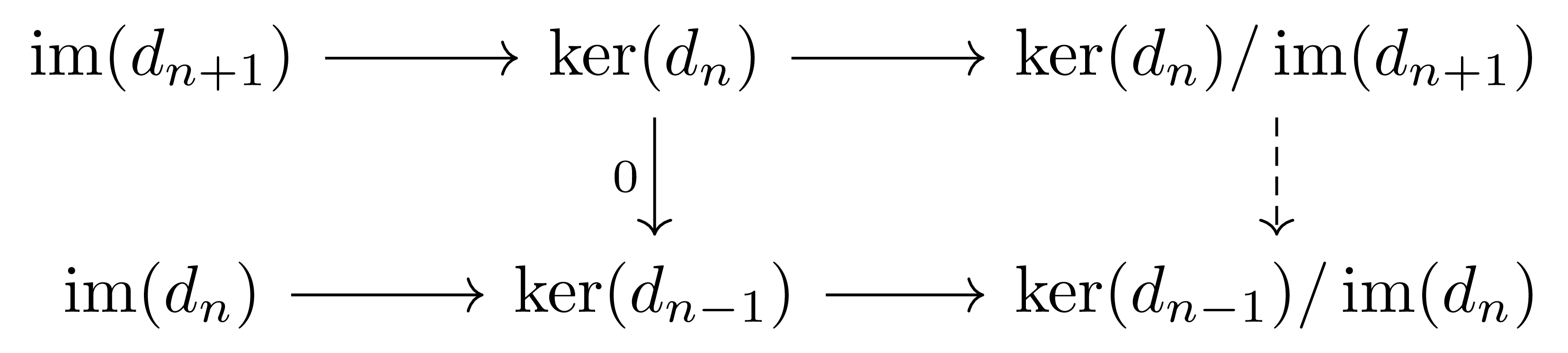
을 통해 유도된다. 그런데 \(\ker(d_n)\rightarrow H_n\)은 epimorphism이고, \(\ker(d_n)\rightarrow\ker(d_{n-1})\)이 \(0\)이므로 \(H_n(C)\rightarrow H_{n-1}(C)\) 또한 zero map이다. 이는 (\(\ker(d_\bullet)\)이나 \(\coker(d_\bullet)\)과 마찬가지로) \(H_\bullet(C)\)가 chain complex로서는 크게 의미가 없고, 대신 \(H_\bullet(C)\)의 각각의 성분인 \(H_n(C)\in\obj(\mathcal{A})\)들이 흥미로운 대상임을 보여준다.
정의 2 임의의 chain complex
\[C_\bullet:\quad\cdots\overset{d_{n+2}}{\longrightarrow} C_{n+1}\overset{d_{n+1}}{\longrightarrow} C_n\overset{d_n}{\longrightarrow} C_{n-1}\overset{d_{n-1}}{\longrightarrow}\cdots\]에 대하여, \(C_\bullet\)의 \(n\)-cycle들의 module은 \(Z_n(C)=\ker (d_n)\)으로 주어진다. 또, \(\im(d_{n+1})\)을 \(C_\bullet\)의 \(n\)-boundary들의 module이라 부르고, \(B_n(C)\)으로 적는다. 이 때, \(C_\bullet\)의 \(n\)번째 호몰로지\(n\)-th homology는 \(H_n(C)=Z_n(C)/B_n(C)\)로 정의된다.
비슷하게 cochain complex에 대해서는 \(n\)-cocycle과 \(n\)-coboundary, 그리고 \(n\)번째 코호몰로지가 정의된다.
\(H_\bullet\) 자체는 \(\Ch(\mathcal{A})\)에서 \(\Ch(\mathcal{A})\)로의 functor지만, 각각의 성분 \(H_n\)은 \(\Ch(\mathcal{A})\)에서 \(\mathcal{A}\)로의 functor를 정의한다.
명제 3 임의의 \(n\)에 대하여, \(H_n\)은 \(\Ch(\mathcal{A})\)에서 \(\mathcal{A}\)로의 functor이다.
증명
임의의 chain map \(f_\bullet:C_\bullet\rightarrow D_\bullet\)에 대하여, §Diagram chasing, ⁋보조정리 4를 적용하면 \(f_n\)이 \(Z_n(C)\rightarrow Z_n(D)\), \(B_n(C)\rightarrow B_n(D)\)을 각각 유도한다는 것을 안다. 따라서 \(f_n\)은
\[H_n(f):H_n(C)\rightarrow H_n(D)\]을 유도한다. 이렇게 얻어지는 데이터들이 functor를 구성한다는 것을 확인하면 되는데, 이는 모두 자명하다.
Double complex와 translation
마지막으로 double complex를 정의한다. 직관적으로 이는 abelian category \(\Ch(\mathcal{A})\)들로 이루어진 chain complex, 즉 \(\Ch(\Ch(\mathcal{A}))\)의 대상이라 생각할 수 있다. 위에서 살펴본 (1)의 chain complex \(C_{\bullet-1}\)과 그 밑의 chain map이 그 예시이다.
그러나 나중에 계산을 할 때 각 행의 부호가 바뀌도록 해주면 더 깔끔한 결과를 얻을 때가 있다.2 이러한 sign convention을 받아들여 다음과 같이 정의한다.
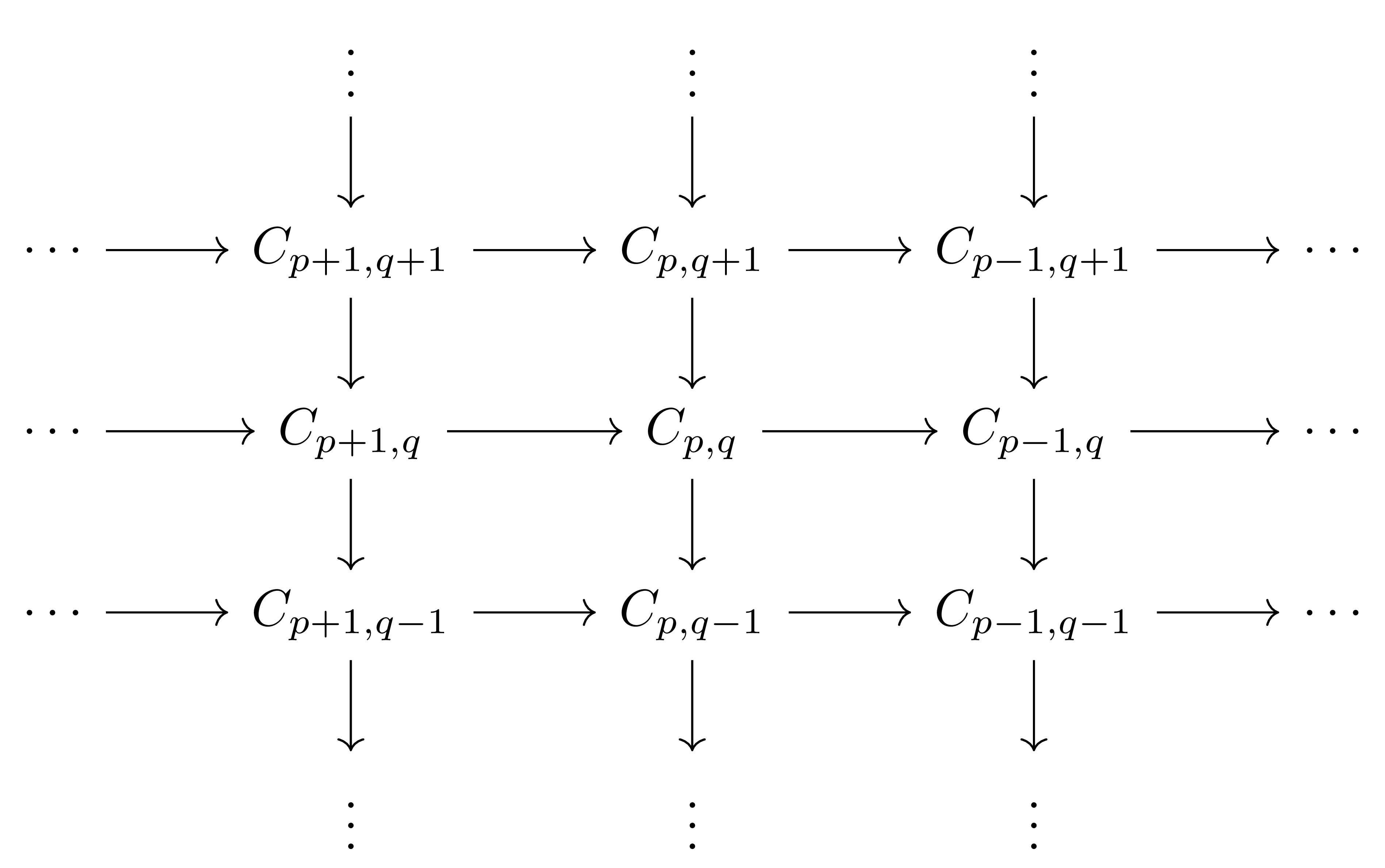
정의 4 Abelian category \(\mathcal{A}\)의 대상들로 이루어진 double complex는 다음의 두 함수들
\[d^h:C_{p,q}\rightarrow C_{p-1,q},\qquad d^v:C_{p,q}\rightarrow C_{p,q-1}\]이 주어진 대상이며, 이들은
\[(d^h)^2=(d^v)^2=d^vd^h+d^hd^v=0\]을 만족한다.
조건 \(d^vd^h+d^hd^v=0\)은 \(d^vd^h=-d^hd^v\)를 의미하므로 double complex들은 \(\Ch(\Ch(\mathcal{A}))\)의 대상이 아니지만, \(d^v\)로부터 다음의 식
\[f_{p,q}=(-1)^pd_{p,q}^v:C_{p,q}\rightarrow C_{p,q-1}\]을 정의하면 이를 \(\Ch(\Ch(\mathcal{A}))\)의 대상으로 취급할 수 있다.
정의 5 Double complex \(C_{p,q}\)의 total complex \(\Tot(C)_\bullet\)는 각 차수 \(n\)에서
\[(\Tot(C))_n = \bigoplus_{p+q=n} C_{p,q}\]로 정의되며, 그 differential은
\[d = d^h + (-1)^p d^v : (\Tot(C))_n \rightarrow (\Tot(C))_{n-1}\]으로 준다. (동등하게 \(d^v + (-1)^q d^h\)로 쓸 수도 있다.)
논의의 편의를 위해 differential을 다소 간략하게 썼지만, 이를 뜯어보면 실제 계산은 위의 식보다는 다소 복잡하다. 가령 double complex \(C_{p,q}\)가 주어졌다 하고, 편의상 이 complex는 \(p,q\geq 0\)인 곳에서만 \(0\)이 아니라 하자. 그럼 이 double complex의 total complex \(\Tot(C)_\bullet\)에서, differential \(d:\Tot(C)_2\rightarrow \Tot(C)_1\)을 계산하려면 다음과 같이 진행해야 한다. 우선 \(\Tot(C)_2\)의 원소는 \((x_{0,2}, x_{1,1}, x_{2,0})\)의 형태이며,3 이 원소의 differential은
\[d^h(x_{0,2})+(-1)^0d^v(x_{0,2})=d^v(x_{0,2}), \quad d^h(x_{1,1})+(-1)^1d^v(x_{1,1}),\quad d^h(x_{2,0})+(-1)^2d^v(x_{2,0})=d^h(x_{2,0})\]의 정보를 모두 담고 있는 다음의 원소
\[(d^v(x_{0,2})+d^h(x_{1,1}), -d^v(x_{1,1})+d^h(x_{2,0}))\in\Tot(C)_1=C_{0,1}\oplus C_{1,0}\]가 된다. 즉, \(\Tot(C)\)는 double complex \(C_{p,q}\)를 하나의 complex로 묶어주는 것이며, 그 과정에서 \(p+q=n\)의 total degree를 갖는 성분들을 모두 동시에 고려해주는 것이다.
이것이 complex임을 보이기 위해서는 \(d^2=0\)을 보여야하는데, 이는 다음의 식
\[(d^h + (-1)^p d^v)^2 = (d^h)^2 + (-1)^p d^vd^h + (-1)^{p-1} d^hd^v + (d^v)^2\]을 통해 얻는다. 여기서 \((d^h)^2=0\), \((d^v)^2=0\)이며, double complex의 조건 \(d^vd^h + d^hd^v=0\)에서 \(d^vd^h = -d^hd^v\)이므로 나머지 두 항도 상쇄된다.
한편, double complex를 정의할 때 위와 같은 sign convention을 사용했으므로, \(C\)의 \(p\)-th translation \(C[p]\) 또한 다음의 식
\[C[p]_n=C_{n+p}\]으로 주어진 chain complex이며, 이 때의 differential은 \((-1)^pd\)으로 정의해야 한다. 예컨대 \(C[-1]\)은 위에서 정의한 \(C_{\bullet-1}\)과 동일하지만, 각 differential들의 부호가 바뀐 chain complex를 의미한다.
어쨌든 이렇게 새로 생겨난 부호와는 관계없이
\[H_n(C[p])=H_{n+p}(C)\]임이 자명하며, 또 만일 \(f:C\rightarrow D\)가 chain map이라면 \(f[p]\)를 다음의 식
\[f[p]_n=f_{n+p}\]으로 정의하여 \(f[p]:C[p]\rightarrow D[p]\)을 만들 수 있다. 즉 translation은 \(\Ch(\mathcal{C})\)에서 자기 자신으로의 functor이다.
Truncation
마지막으로 임의의 chain complex \(C_\bullet\)가 주어졌다 하자. 임의의 정수 \(n\)에 대하여, 다음의 식
\[(\tau_{\geq n}C)_i=\begin{cases}0&\text{if $i < n$}\\ Z_n&\text{if $i=n$}\\ C_i&\text{if $i > n$}\end{cases}\]그리고 \(C_\bullet\)와 동일한 differential로 정의된 chain complex \((\tau_{\geq n}C)_\bullet\)를 intelligent truncation이라 부른다. 그럼
\[H_i(\tau_{\geq n}C)=\begin{cases}0&\text{if $i < n$}\\ H_i(C)&\text{if $i\geq n$}\end{cases}\]이 된다. 비슷하게 \((\tau_{< n}C)_\bullet\) 또한 정의할 수 있다. 한편 Brutal truncation은 다음의 식
\[(\sigma_{\geq n}C)_i=\begin{cases}0&\text{if $i \leq n$}\\ C_i&\text{otherwise}\end{cases}\]으로 정의된다. 정의 자체는 \((\sigma_{\geq n}C)_\bullet\)가 더 자연스러워보일 수 있지만, \(n\)번째 호몰로지를 살펴보면 intelligent truncation이 더 좋은 연산을 준다는 것을 확인할 수 있다.
참고문헌
[Wei] C.A. Weibel. An Introduction to Homological Algebra. Cambridge Studies in Advanced Mathematics. Cambridge University Press, 1995.
[Hu] S.T. Hu, Introduction to homological algebra. University Microfilms, 1979.
-
여기에서 \(\oplus\)는 \(\mathcal{A}\)에서의 coproduct인 것으로 이해한다. Abelian category에서
유한한 대상들의 product와 coproduct는 일치한다는 것을 증명할 수 있으므로, 사실 \(A\oplus B\cong A\times B\)이다. ↩ -
예를 들어, Dolbeault operator \(d=\partial+\bar{\partial}\)의 경우 \(d^2=0\)은 \(0=\partial^2+(\partial\bar{\partial}+\bar{\partial}\partial)+\bar{\partial}^2\)와 같으며, bidegree를 고려해주면 \(\partial\bar{\partial}+\bar{\partial}\partial=0\)임을 안다. ↩
-
편의상 \(p,q\geq 0\)인 곳에서만 \(C_{p,q}\neq 0\)이라 가정했으므로 가령 \(x_{-1,3}\)과 같은 항은 무시해도 된다. ↩
댓글남기기