Characteristic Classes

This post was translated from Korean by LLM (Kimi). The translation may contain errors or awkward sentences. The Korean original is the source of truth.

In the previous post, the map \(p:\Spe(\or_M^A)\rightarrow M\) played an important role as a covering space, and these satisfied the following properties.

1. For any \(x\in M\), we have \(p^{-1}(x)\cong \{x\}\times A^\times\).
2. Moreover, for any \(x\in M\), there exists a suitable open set \(U\) such that \(p^{-1}(U)\cong U\times A^\times\).

Now we generalize this further and examine the case where \(p^{-1}(x)\) carries additional structure (other than being a discrete set). The most general definition is as follows.

Definition 1 For a continuous surjection \(p:E \rightarrow B\) between topological spaces and a topological space \(F\), a fiber bundle is a structure for which, for each \(x\in B\), there exists an open set \(U\) and a homeomorphism \(\phi:U\times F\rightarrow p^{-1}(U)\) making the following diagram

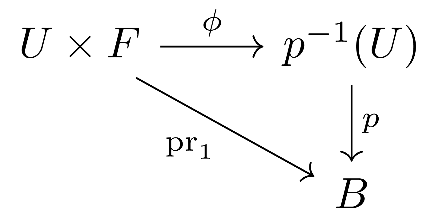
commute.

In this case, \(B\) is called the base space of this bundle, \(E\) the total space, and \(F\) the fiber. If we can choose \(U=B\), then this fiber bundle is called a trivial bundle. For instance, in the preceding example, \(M\) is the base space, \(\Spe(\or_M^A)\) is the total space, and \(A^\times\) equipped with the discrete topology is the fiber. More generally, any covering space can be regarded as a fiber bundle whose fiber is equipped with the discrete topology.

The two cases of particular interest to us are when the fiber \(F\) is a vector space and when it is a topological group. For convenience, we shall assume from now on that \(B\) is connected.

Vector Bundles

First we consider the case where \(F\) is a vector space. When the fiber \(F\) is a topological group, it is already endowed with a topology, so the topology on the product space \(U\times F\) in Definition 1 is clear; however, when \(F\) is a vector space, this is somewhat ambiguous. The most general setting would use the notion of a topological vector space \(V\) on which a topological ring \(\mathbb{K}\) acts, but for convenience we shall for now only consider the case where the base field of \(F\) is \(\mathbb{R}\) and \(F\) is equipped with the metric topology arising from the canonical inner product.

Definition 2 For a fiber bundle \(p:E \rightarrow B\), the fiber space \(F\) is an \(\mathbb{R}\)-vector space equipped with a topology as above, and additionally, for any \(x\in B\) and the homeomorphism \(\phi:U\times F\rightarrow p^{-1}(U)\) from Definition 1, the following function

\[\phi(x,-):F \rightarrow p^{-1}(x);\qquad v\mapsto \phi(x,v)\]

is an isomorphism of vector spaces.

Through this, each fiber \(p^{-1}(x)\) inherits a vector space structure from \(F\). In general, given two vector bundles \(p_1:E_1 \rightarrow B_1\) and \(p_2:E_2\rightarrow B_2\), a morphism between them is a commutative diagram of continuous functions

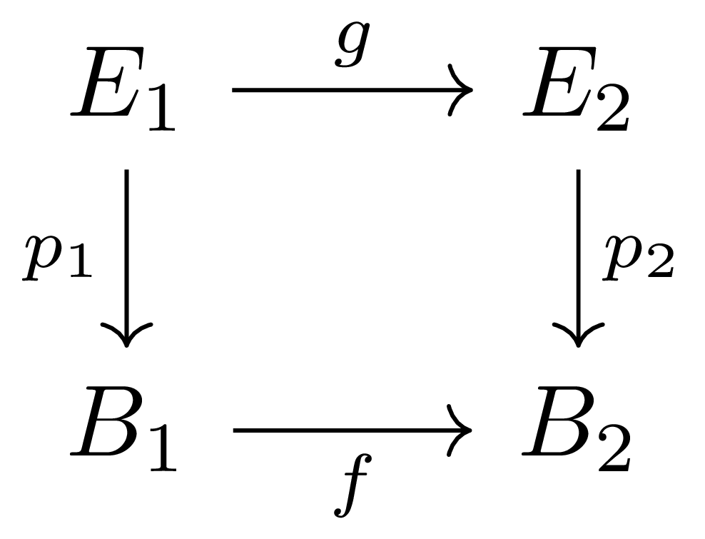
Here, the restriction of \(g\) to \(p^{-1}(x)\rightarrow p_2^{-1}(f(x))\) for each \(x\in B_1\) must be a linear map between vector spaces. It is obvious how to define isomorphisms between vector bundles.

Meanwhile, in Definition 2 above, we only considered the case where \(F\) is an \(\mathbb{R}\)-vector space, and defined a topology on it using the inner product structure on \(\mathbb{R}^n\) and the topology of \(\mathbb{R}\). However, strictly speaking, the only information needed here is the topology of the vector space \(F\), and when \(F\) is regarded as an inner product space, this is called a Euclidean bundle. Anyway, since we will mostly only think about \(\mathbb{R}\)-vector spaces, we shall gloss over this distinction.

Example 3 A non-trivial example is the orientation double cover of the Möbius strip. Meanwhile, in §Poincaré Duality, ⁋Example 3 we also considered a non-trivial cover of \(S^1\), which can be generalized geometrically as follows.

For an \((n+1)\)-dimensional vector space \(\mathbb{R}^{n+1}\), we call the space of lines through the origin the projective \(n\)-space and denote it by \(\RP^n\). Among the points on a line through the origin, the two points at distance \(1\) from the origin specify the same line; thus we may think of this as the quotient space obtained by identifying antipodal points on the unit \(n\)-sphere \(S^n\).

Now let us take this space \(\RP^n\) as the base space \(B\), and define the vector bundle \(E(\gamma_n^1)\) over it as follows. As a set,

\[E(\gamma_n^1)=\{((x,v)\in \RP^n\times \mathbb{R}^{n+1}\mid x\in \span(x)\}\]

it is defined as above, and the projection \(\gamma_n^1:E(\gamma_n^1)\rightarrow \RP^n\) is the projection onto the first coordinate. In other words, \(\gamma_n^1\) attaches to each point \(x\in \RP^n\) exactly the line in \(\mathbb{R}^{n+1}\) to which \(x\) originally belonged.

This is not a trivial bundle. If it were a trivial bundle, there would exist a non-vanishing continuous section \(\RP^n\rightarrow E(\gamma_n^1)\). For instance, the function assigning the element \(1\) in the fiber to every point of \(B\) would be such a section. However, given any section \(s:\RP^n \rightarrow E(\gamma_n^1)\), consider the following composition using the quotient map \(q:S^n \rightarrow \RP^n\):

\[S^n \overset{q}{\longrightarrow} \RP^n \overset{s}{\longrightarrow} E\overset{\pr_2}{\longrightarrow} \mathbb{R}^{n+1}\]

This function sends \(\mathbf{x}\in S^n\subset\mathbb{R}^{n+1}\) to a scalar multiple of \(\mathbf{x}\). Denoting this scalar by \(t(\mathbf{x})\), we see that \(t\) is a continuous function from \(S^n\) to \(\mathbb{R}\), and because of the quotient map \(q\),

\[t(-\mathbf{x})=-t(\mathbf{x})\]

it satisfies. Since \(S^n\) is connected, the intermediate value theorem implies that there exists \(\mathbf{x}_0\in S^n\) such that \(t(\mathbf{x}_0)=0\).

More generally, the following holds.

Proposition 4 For a vector bundle \(E\) of rank \(n\) over a topological space \(B\), \(E\) is a trivial bundle if and only if there exist \(n\) everywhere linearly independent sections \(s_1,\ldots, s_n\).

Meanwhile, given any vector bundle \(p:E \rightarrow B\) and any continuous map \(f:B'\rightarrow B\), we define the expression

\[f^\ast E=\{(x,v)\in B'\times E\mid f(x)=p(v)\}\subset E\]

as \(f^\ast E\), thereby defining a new vector bundle \(f^\ast E \rightarrow B'\). We call this the pullback bundle, and it is not hard to see that if any vector bundle \(E' \rightarrow B'\) satisfies the above condition, then it factors through \(f^\ast E\).

Meanwhile, given any two vector bundles \(p_1:E_1\rightarrow B_1\) and \(p_2:E_2\rightarrow B_2\), their product

\[p_1\times p_2: E_1\times E_2 \rightarrow B_1\times B_2\]

is also a vector bundle over \(B_1\times B_2\). Now if \(B_1=B_2=B\), then as always the diagonal map

\[\Delta: B\rightarrow B\times B\]

gives the pullback bundle \(\Delta^\ast(p_1\times p_2)\), which becomes a bundle over \(B\). We call this the Whitney sum of the two vector bundles \(E_1\rightarrow B\) and \(E_2\rightarrow B\), and denote it by \(p_1\oplus p_2:E_1\oplus E_2\rightarrow B\). As the notation suggests, this corresponds fiberwise to the direct sum of the fibers of the two vector bundles \(E_1\) and \(E_2\).

Although we have not given detailed proofs, in a similar way we can lift operations defined on each fiber (that is, on the vector space) to the vector bundle. For example, for two vector bundles \(E_1\rightarrow B\) and \(E_2 \rightarrow B\), we can form their tensor product bundle \(E_1\otimes E_2 \rightarrow B\), and it is also possible to use operations such as \(\Hom\) or \(\bigwedge\).

Čech Cohomology

At this point we establish yet another cohomology theory. Like sheaf cohomology (§Poincaré Duality, ⁋Definition 14), this is a cohomology of sheaves defined on a topological space, and because via the étale space construction we can regard sheaves whose stalks are vector spaces as the same thing as vector bundles, it plays an important role in our story. Sheaf cohomology showed that cohomology encodes the obstructions to the existence of global sections of a sheaf. The Čech cohomology we are about to examine yields similar results, but differs in that it seeks the answer by examining the process of patching local sections together to make a global section. In any case, in good cases including manifolds, Čech cohomology gives the same results as sheaf cohomology, and hence the Čech cohomology of a constant sheaf recovers the cohomology we originally knew.

Consider a topological space \(X\), a sheaf \(\mathscr{F}\) defined on it, and an open cover \(\mathcal{U}=\{U_i\}_{i\in I}\) of \(X\). For each \(p\geq 0\), the group of Čech \(p\)-cochains is given by the formula

\[\check{C}^p(\mathcal{U},\mathscr{F})=\prod_{i_0,\ldots,i_p}\mathscr{F}(U_{i_0}\cap \cdots\cap U_{i_p})\]

is defined as. That is, this is the collection of sections defined over all such intersections. The differential

\[\check{C}^p(\mathcal{U},\mathscr{F})\rightarrow \check{C}^{p+1}(\mathcal{U}, \mathscr{F})\]

is given by the formula

\[(\delta c)_{i_0,\ldots, i_{p+1}}=\sum_{k=0}^{p+1} (-1)^k c_{i_0,\ldots,\hat{i}_k,\ldots,i_{p+1}}\vert_{U_{i_0}\cap\cdots\cap U_{i_{p+1}}}\]

Then Čech cohomology is given by the formula

\[\check{H}^p(\mathcal{U}, \mathscr{F})=\frac{\ker(\check{C}^p\rightarrow \check{C}^{p+1})}{\im(\check{C}^{p-1}\rightarrow \check{C}^{p})}\]

If \(\mathcal{U}\) is a sufficiently good cover, for instance if every finite intersection is contractible or is acyclic for \(\mathscr{F}\), then we obtain a canonical isomorphism

\[H^p(X,\mathscr{F})\cong \check{H}^p(\mathcal{U},\mathscr{F})\]

Now any rank \(n\) vector bundle is determined by how its fibers are glued over an open cover. That is, by functions

\[g_{ij}:U_{ij}=U_i\cap U_j \rightarrow \GL(n;\mathbb{R})\]

These must satisfy the following condition

\[g_{ij}\cdot g_{jk}\cdot g_{ki}=\id\]

If this condition were absent, it would mean that over the triple intersection \(U_i\cap U_j\cap U_k\), bringing the local trivialization of \(U_i\) to \(U_j\) via \(g_{ij}\), then to \(U_k\) via \(g_{jk}\), and back to \(U_i\) via \(g_{ki}\), the trivialization would have changed, whereas in reality it does not. Then the transition functions \(g_{ij}\) become Čech 1-cochains, and thus, once local trivializations \(U_i\rightarrow \GL(n;\mathbb{R})\) are fixed, we see that there is a one-to-one correspondence between isomorphism classes of rank \(n\) vector bundles and 1-cochains. In other words, there is a one-to-one correspondence between isomorphism classes of rank \(n\) vector bundles trivializable over the open cover \(\mathcal{U}\) and \(\check{H}^1(\mathcal{U}, \GL(n;\mathbb{R}))\).

Earlier, in §Poincaré Duality, ⁋Proposition 4, we saw that the \(A\)-orientability of a manifold \(M\) is defined by the following group homomorphism

\[\pi_1(M,x)\rightarrow A^\times\]

Since \(A\) is a commutative ring, the above group homomorphism factors through the following abelian group homomorphism

\[H_1(M)\rightarrow A^\times\]

and by §Cohomology, ⁋Proposition 3 this is an element of \(H^1(M;A)\). If this element is zero, this is equivalent to the monodromy action being trivial, which means that \(\Spe(\or_M^A)\) is a trivial covering space, so that \(M\) becomes an \(A\)-orientable manifold. On the other hand, for any commutative ring \(A\), since the initial object of \(\cRing\) is \(\mathbb{Z}\), once a \(\mathbb{Z}\)-orientation \(H_1(M)\rightarrow \mathbb{Z}^\times\) is determined for any manifold \(M\), we can compose it with \(\mathbb{Z}^\times\rightarrow A^\times\) to determine an \(A\)-orientation \(H_1(M)\rightarrow A^\times\). Therefore, we know that the essential information about whether \(\Spe(\or_M^A)\) is a trivial cover lies in \(H^1(M;\mathbb{Z}/2)\), and thinking of \(\mathbb{Z}/2\) as \(\GL(1;\mathbb{Z})\), this is an example of how first cohomology contains information about covering spaces.

In this way, information about a vector bundle \(E\rightarrow B\) of rank \(k\) can be regarded as being contained in \(\check{H}^1(B; \underline{\GL(k,\mathbb{R})})\). However, since the coefficients in the cohomology of \(B\) that we use are \(\mathbb{Z}\), we do not possess all the data contained there. Instead, our goal is to find objects that can weakly replace this, namely invariants in the cohomology ring \(H^\bullet(B)\).

Stiefel-Whitney Classes

The first characteristic class we examine is the Stiefel-Whitney class. First, for any vector bundle \(p:E\rightarrow B\), this is an element \(w(p)\) of the cohomology ring \(H^\bullet(B;\mathbb{Z}/2)\), and as above, if \(w(p)=0\) then \(E\) becomes a trivial bundle. That is, if \(w(p)=0\), then by Proposition 4 there exist \(n=\rank(E)\) everywhere linearly independent continuous sections. Moreover, decomposing \(w(p)\) according to the degree in the cohomology ring as

\[w(p)=w_0(p)+w_1(p)+\cdots\]

each \(w_i(p)\) becomes an obstruction class to choosing \(n-i+1\) everywhere linearly independent sections. That is, if \(w_i(p)\neq 0\), then \(n-i+1\) everywhere linearly independent sections cannot exist. In particular, if \(w_n(p)\neq 0\), then not even a single everywhere linearly independent section can exist, so any section must vanish somewhere.

For convenience, when the projection map \(p\) and the base \(B\) are clear, we sometimes use notation such as \(w(E)\) instead of \(w(p)\). Now we present the axioms satisfied by \(w(E)\).

Definition 5 For a vector bundle \(E \rightarrow B\) of rank \(n\) and a vector bundle \(F\rightarrow B\), cohomology classes \(w_i(E)\in H^i(B;\mathbb{Z}/2)\) satisfying the following axioms are called the Stiefel-Whitney classes.

1. (Rank) \(w_0(E)=1\), and if \(i>n\) then \(w_i(E)=0\).
2. (Naturality) For any \(f:B'\rightarrow B\), we have \(w(f^\ast E)=f^\ast w(E)\).
3. (Whitney product formula) We have \(w(E\oplus F)=w(E)w(F)\).
4. (Normalization) For the tautological line bundle \(\gamma_1^1:E(\gamma_1^1)\rightarrow \RP^1\) of Example 3, we have \(w_1(\gamma_1^1)\neq 0\).

Then the following results are obvious.

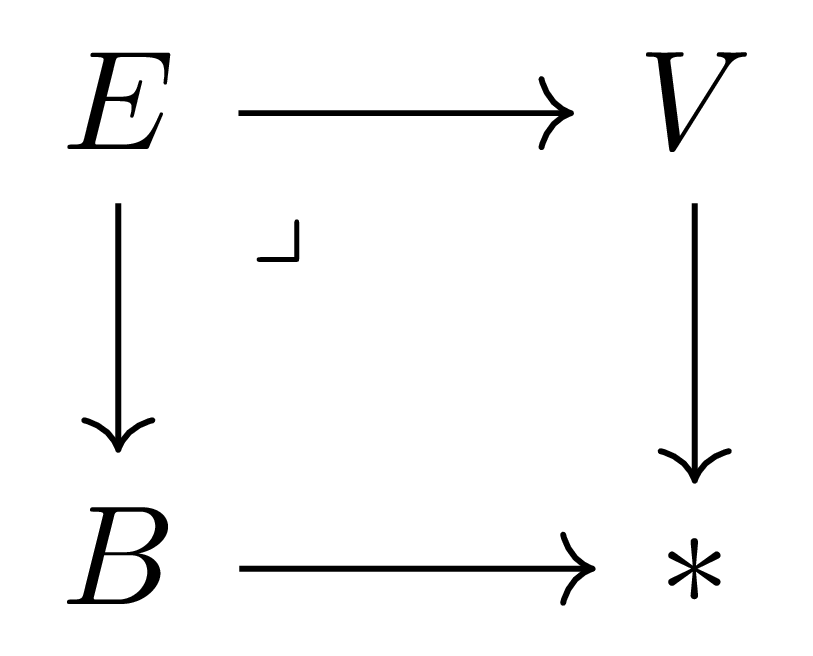
Proposition 6 For two vector bundles \(p_1:E_1\rightarrow B_1\) and \(p_2:E_2\rightarrow B_2\), if \(p_1\) and \(p_2\) are isomorphic then \(w(E_1)=w(E_2)\). In particular, if \(p:E\rightarrow B\) is a trivial bundle then \(w(E)=0\).

The first claim is obvious. For the second claim, it suffices to check that the trivial bundle is given by the following pullback:

An interesting observation is that there are only two isomorphism classes of line bundles over \(S^1\): the trivial line bundle and the line bundle of Example 3. Indeed, among line bundles over \(S^1\), the line bundle obtained by “twisting twice” can be checked to be isomorphic to the trivial line bundle. This is somewhat predictable from Proposition 6, because the Stiefel-Whitney class of a line bundle over \(S^1\) must lie in \(H^1(S^1;\mathbb{Z}/2)\), which is isomorphic to \(\mathbb{Z}/2\).

These are pullbacks of the tautological line bundle over \(\RP^1\). The trivial line bundle over \(S^1\) is the pullback via the continuous map sending every point of \(S^1\) to a fixed point of \(\RP^1\), and the nontrivial line bundle is the pullback of the line bundle via the quotient map \(S^1 \rightarrow \RP^1\).

Grassmannians

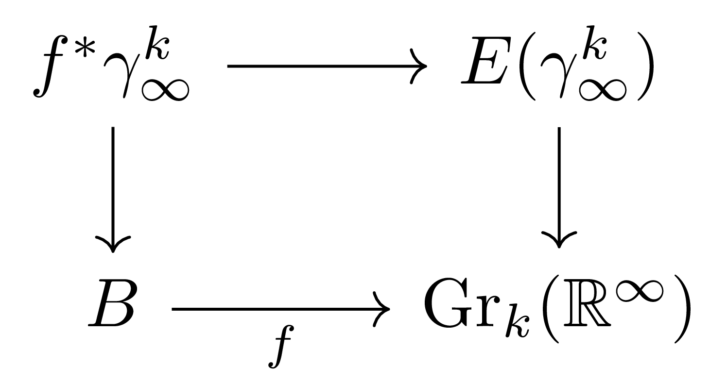
More generally, any rank \(k\) vector bundle over any space is obtained by pulling back the universal bundle \(\gamma^k_\infty:E(\gamma_\infty^k)\rightarrow \Gr_k(\mathbb{R}^\infty)\) over the infinite Grassmannian \(\Gr_k(\mathbb{R}^\infty)\). That is, given any vector bundle \(p:E \rightarrow B\), there exists a unique bundle map from \(p\) to \(\gamma_k^\infty\) making the following diagram commute:

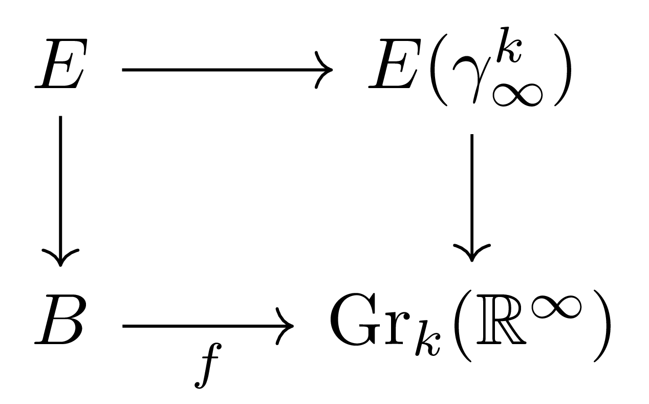
and this is isomorphic to the following pullback diagram:

Moreover, the Stiefel-Whitney classes of the vector bundle \(E\) are also obtained by pulling back the Stiefel-Whitney classes \(w(\gamma^k_\infty)\) of the universal bundle \(\gamma^k_\infty\). Therefore, we must examine the (infinite) Grassmannian and the universal bundle over it, as well as the cohomology ring \(H^\bullet(\Gr_k(\mathbb{R}^\infty), \mathbb{Z}/2)\) of the infinite Grassmannian in which the Stiefel-Whitney classes of this bundle live. Since it is a complicated task to prove all the properties of Grassmannians rigorously, in this section we shall content ourselves with an introduction to these properties and, where possible, a brief explanation.

First we examine the basic properties and the cohomology ring of \(\Gr_k(\mathbb{R}^n)\). By definition, \(\Gr_k(\mathbb{R}^{n})\) is the space of all \(k\)-dimensional linear subspaces of \(\mathbb{R}^{n}\). For example, \(\Gr_1(\mathbb{R}^{n+1})\) is by definition the projective space \(\RP^n\). Since each point of \(\Gr_k(\mathbb{R}^{n})\) is a subspace of \(\mathbb{R}^{n}\), we intuitively know how close two points (that is, two \(k\)-dimensional subspaces of \(\mathbb{R}^{n}\)) are to each other. This is the same phenomenon as, for example, points corresponding to two lines with similar “slopes” in \(\mathbb{R}^{n+1}\) being close in \(\RP^n\). This can be defined rigorously using \(n\times k\) matrices, and with this topology \(\Gr_k(\mathbb{R}^{n})\) becomes a \(k(n-k)\)-dimensional compact topological manifold.

Now let us examine their cohomology ring. Since we are using \(\mathbb{Z}/2\)-coefficients anyway, by §Poincaré Duality, ⁋Theorem 11 we may think in terms of homology cycles of \(\Gr_k(\mathbb{R}^n)\). To this end, fix a full flag of \(\mathbb{R}^n\)

\[F_\bullet:\qquad 0=F_0\subset F_1\subset F_2\subset\cdots\subset F_n=\mathbb{R}^n\]

Then for any \(k\)-plane \(X\) in \(\mathbb{R}^n\),

\[0=\dim (X\cap F_0)\leq\dim(X\cap F_1)\leq\cdots\leq \dim(X\cap F_n)=k\]

is defined, and this sequence shows how \(X\) sits inside \(\mathbb{R}^n\). To track this, we define a Schubert symbol \(\sigma=(\sigma_1,\ldots, \sigma_k)\) as a sequence satisfying the following condition

\[1\leq \sigma_1<\sigma_2<\cdots<\sigma_k\leq n\]

These \(\sigma_i\) indicate when the space \(X\cap F_i\) grows. That is, they are

\[\dim(X\cap F_{\sigma(i)})=i, \qquad \dim(X\cap F_{\sigma(i)-1})=i-1\]

can contain the information measuring where the dimension jumps. Reversing this, we can encode this information via a suitable partition

\[\lambda:\qquad \lambda_1\geq\lambda_2\geq\cdots\geq\lambda_k,\qquad \lambda_1\leq n-k\]

with the following condition

\[\dim(X\cap F_{n-k+i-\lambda_i})\geq i\]

These partitions, for a fixed flag

\[F_0\subset F_1\subset\cdots\subset F_n\]

show when the dimension of \(X\cap F_i\) jumps. For example, when \(X=F_k\), the corresponding partition is \((0,0,\ldots,0)\), which means that the \(X\cap F_i\) complete all their dimension jumps without delay in the first \(k\) terms as \(i\) increases. For instance, \((0,1,0,\ldots,0)\) means that \(X\cap F_1\) is 1-dimensional, \(X\cap F_2\) is also 1-dimensional, \(X\cap F_3\) is 2-dimensional, and after that the dimensions jump by one without delay.

Now based on this, consider the following subset

\[\Omega_\lambda^\circ(F_\bullet)=\left\{V\in\Gr_k(F_n)\mid\text{$\dim(V\cap F_{n-k+i-\lambda_i})= i$ for all $1\leq i\leq k$}\right\}\]

Then each of these is an open submanifold inside its closure

\[\Omega_\lambda(F_\bullet)=\left\{V\in\Gr_k(F_n)\mid\text{$\dim(V\cap F_{n-k+i-\lambda_i})\geq i$ for all $1\leq i\leq k$}\right\}\]

and these \(\Omega_\lambda(F_\bullet)\) define homology classes of \(\Gr_k(\mathbb{R}^n;\mathbb{Z}/2)\) via the inclusion

\[\Omega_\lambda(F_\bullet)\hookrightarrow \Gr_k(\mathbb{R}^n)\]

We call these Schubert cycles, and their Poincaré duals \(\sigma_\lambda\) are called Schubert classes. These are cohomology classes of degree \(\lvert \lambda\rvert=\sum \lambda_i\). At this point, the subspaces \(\Omega_\lambda(F_\bullet)\) depend on the choice of flag \(F_\bullet\), but the Schubert cycles, being their images in homology, do not depend on the choice of \(F_\bullet\), and consequently neither do the Schubert classes. Moreover, \(H^\bullet(\Gr_k(\mathbb{R}^n);\mathbb{Z}/2)\) is the polynomial algebra generated by the partitions \(\lambda\) satisfying the above conditions, and therefore it suffices to look at the cup product structure among them.

Example 7 For example, consider \(\Gr_2(\mathbb{R}^4;\mathbb{Z}/2)\). Here we shall examine the square of the Schubert class \(\sigma_{(1,0)}\) corresponding to the partition \((1,0)\),

\[\sigma_{(1,0)}\smile\sigma_{(1,0)}=\sigma_{(1,1)}+\sigma_{(2,0)}\]

To utilize our geometric intuition, let us think of this as an intersection of Schubert cycles, as in §Poincaré Duality, ⁋Example 15. For this, we need to consider two subspaces in general position among the homology classes corresponding to \(\sigma_{(1,0)}\), and this is possible by changing the choice of flag.

For a fixed flag \(F_\bullet\), let us explicitly write out the condition represented by the partition \(\lambda=(1,0)\). It is the following condition:

\[\dim(X\cap F_{4-2+1-1})=\dim(X\cap F_2)\geq 1,\qquad \dim(X\cap F_{4-2+2-0})=\dim (X\cap F_4)\geq 2\]

That is, the only effectively nontrivial condition is \(\dim(X\cap F_2)\geq 1\). In other words, this means that \(X\) meets \(F_2\) in dimension at least 1, which can be rephrased as the condition that \(X\) contains a suitable line \(L\) contained in \(F_2\).

Now to compute the cup product \(\sigma_{(1,0)}\smile\sigma_{(1,0)}\), we need to consider two flags \(F_\bullet\) and \(F_\bullet'\) in general position. For example,

\[F_\bullet:\quad \langle e_1\rangle\subset \langle e_1,e_2\rangle\subset \langle e_1,e_2,e_3\rangle,\qquad F_\bullet':\quad \langle e_4\rangle\subset \langle e_3,e_4\rangle\subset \langle e_2,e_3,e_4\rangle\]

satisfy this. Now the \(V\) we consider must meet both \(\langle e_1,e_2\rangle\) and \(\langle e_3,e_4\rangle\) in dimension 1. For this, consider another flag

\[G_\bullet:\quad \langle e_1+e_4\rangle\subset\langle e_1+e_4,e_2+e_3\rangle\subset \langle e_1+e_4,e_2+e_3,e_2-e_3\rangle\]

Then there are two cases. First, one case is when the plane spanned by the two lines of \(F_2\) and \(F_2'\) is not contained in \(G_3\). For example, the case where \(V\) meets \(F_2\) at \(\span(e_1+e_2)\) and \(V\) meets \(F_2'\) at \(\span(e_3+e_4)\) corresponds to this. In this case, \(V\) can be written exactly as \(\span(e_1+e_2,e_3+e_4)\), which meets \(G_0\) and \(G_1\) in dimension 0, \(G_2\) and \(G_3\) in dimension 1, and finally \(G_4\) in dimension 2. That is, this corresponds to \((1,1)\).

The other case is when the plane spanned by the two lines of \(F_2\) and \(F_2'\) is contained in \(G_3\). For instance, if we consider the case where \(V\) meets \(F_2\) at \(\span(e_2)\) and \(V\) meets \(F_3\) at \(\span(e_3)\), then \(V=\span(e_2,e_3)\), which is contained in \(G_3\). This case corresponds to \((2,0)\).

More generally, we can represent these partitions by Young diagrams, and using these we can compute the coefficient appearing in front of \(\sigma_\nu\) for \(\nu\) satisfying \(\lvert\nu\rvert=\lvert\lambda\rvert+\lvert\mu\rvert\) when we compute the cup product \(\sigma_\lambda\smile\sigma_\mu\) of two Schubert classes.

Now we must define \(\Gr_k(\mathbb{R}^\infty)\) and the universal bundle over it. For this, we first define the tautological bundle over \(\Gr_k(\mathbb{R}^n)\). As in Example 3, the following bundle attaches to each point of \(\Gr_k(\mathbb{R}^{n+k})\) the vector space corresponding to that point:

\[E(\gamma^k_n)=\left\{([V], x)\in \Gr_k(\mathbb{R}^{n+k})\mid \text{$V$ a $k$-dimensional subspace of $\mathbb{R}^{n+k}$ and $x\in V$}\right\}\]

exists, and we call it the tautological bundle over \(\Gr_k(\mathbb{R}^{n+k})\). Now for each \(n\), the formula

\[\mathbb{R}^{k+n} \rightarrow \mathbb{R}^{k+n+1};\qquad (x_1,\ldots,x_{k+n}) \mapsto (x_1,\ldots,x_{k+n},0)\]

defines an inclusion of \(\mathbb{R}^{k+n}\) into \(\mathbb{R}^{k+n+1}\), and through this we can view a \(k\)-dimensional subspace of \(\mathbb{R}^{k+n}\) as a \(k\)-dimensional subspace of \(\mathbb{R}^{k+n+1}\). That is, the above inclusion induces an inclusion \(\Gr_k(\mathbb{R}^{k+n})\rightarrow \Gr_k(\mathbb{R}^{k+n+1})\) between Grassmannians. Now consider the following directed system

\[\Gr_k(\mathbb{R}^k)\hookrightarrow \Gr_k(\mathbb{R}^{k+1})\hookrightarrow\cdots\]

Then their direct limit

\[\Gr_k(\mathbb{R}^\infty)=\varinjlim_{n\geq 0}\Gr_k(\mathbb{R}^{k+i})\]

is called the infinite Grassmannian. In the same way, the direct limit of total spaces

\[E(\gamma_\infty^k)=\varinjlim_{n\geq 0} E(\gamma^k_{k+n})\]

is defined, and this defines a rank \(k\) vector bundle over \(\Gr_k(\mathbb{R}^\infty)\). Of course, these do not depend on the choice of inclusion \(\mathbb{R}^{k+n}\hookrightarrow \mathbb{R}^{k+n+1}\).

Intuitively, \(\Gr_k(\mathbb{R}^\infty)\) can be thought of as attaching the various \(\Gr_k(\mathbb{R}^{k+n})\) together to give a CW-complex structure. Moreover, the tautological bundles \(E(\gamma^k_{n+k})\) are attached in a way compatible with this structure. It is not straightforward to transfer the Schubert classes of finite Grassmannians to the infinite Grassmannian. However, as explained above, the infinite Grassmannian is a space having the finite Grassmannians as subcomplexes, and the Schubert cycles constructed above behave well with respect to these inclusions. That is, pushing forward the Schubert cycle of \(\Gr_k(\mathbb{R}^{k+i})\) corresponding to the partition \(\lambda\) via \(\Gr_k(\mathbb{R}^{k+i})\rightarrow \Gr_k(\mathbb{R}^{k+i+1})\) gives the same result as intersecting the Schubert cycle corresponding to the partition \(\lambda\) in \(\Gr_k(\mathbb{R}^{k+i+1})\) directly with \(\Gr_k(\mathbb{R}^n)\subset \Gr_k(\mathbb{R}^{k+i+1})\).

Now consider the \(k\) partitions

\[\lambda_1=(1,0,\cdots, 0),\quad \lambda_2=(2,0,\cdots,0),\qquad \lambda_k=(k,0,\cdots,0)\]

Then by the above argument these become homology classes of \(\Gr_k(\mathbb{R}^\infty)\), and the following functions

\[w_i: H_\bullet(\Gr_k(\mathbb{R}^\infty);\mathbb{Z}/2)\rightarrow \mathbb{Z}/2; \qquad \text{$w_i(\Omega_{\lambda_i}(F_\bullet))=1$ and is 0$ otherwise}\]

lie in the \(i\)-th cohomology \(H^i(\Gr_k(\mathbb{R}^\infty);\mathbb{Z}/2)\), and therefore we have

\[w_1\in H^1(\Gr_k(\mathbb{R}^\infty);\mathbb{Z}/2),\cdots, w_k\in H^k(\Gr_k(\mathbb{R}^\infty);\mathbb{Z}/2)\]

Then \(H^\bullet(\Gr_k(\mathbb{R}^\infty);\mathbb{Z}/2)\) is generated as a polynomial algebra by these $$w_i