Homotopy

Topological Invariants

In general, given mathematical objects, we are interested in classifying them (with respect to isomorphism). For instance, sets are completely classified by their cardinality, and \(\mathbb{k}\)-vector spaces are completely classified by their dimension. However, in most cases such classification is not an easy task, and topological spaces are no exception.

The homologies of topological spaces defined in our previous posts are topological invariants due to functoriality. That is, if two topological spaces \(X\) and \(Y\) are homeomorphic, then they are also homologous. However, the converse does not hold in general. While finding a topological invariant that completely determines a topological space might be one of our goals, there is the following interesting result.

Theorem 1 (Markov 1958) There is no finite algorithm that determines whether two topological manifolds of dimension 4 or higher are homeomorphic to each other.

Naïvely speaking, if there exists a topological invariant that tells us whether arbitrary topological spaces are homeomorphic, then there is generally no appropriate method to compute this invariant. From this perspective, topological invariants are useful only for showing that two topological spaces are not homeomorphic, rather than for proving that they are homeomorphic.

Homotopy Equivalence

The homotopy equivalence that we will introduce in this post is similarly useful for showing that two topological spaces are not homeomorphic, and moreover, it is finer than the equivalence defined by homology. That is, the following implication

\[X,Y\text{ homeomorphic}\implies X,Y \text{ homotopically equivalent}\implies X,Y\text{ homologous}\tag{$\ast$}\]

holds, but its converse does not. Furthermore, homotopy equivalence is geometrically more intuitive compared to homology.

Definition 2 Let \(f_0,f_1:X \rightarrow Y\) be continuous functions between two topological spaces \(X,Y\). We say that \(f_0\) and \(f_1\) are homotopic if there exists a continuous function \(F:X\times [0,1]\rightarrow Y\) such that the two equations

\[F(x,0)=f_0(x),\qquad F(x,1)=f_1(x)\tag{1}\]

hold for all \(x\in X\). In this case, \(F\) is called a homotopy between \(f_0\) and \(f_1\), and if a homotopy exists between \(f_0\) and \(f_1\), we write \(f_0\simeq f_1\).

Intuitively, this means that \(f_0\) can be continuously deformed to obtain \(f_1\). In the above definition, giving a continuous function \(F\) is equivalent to giving a family \((F(-,t))_{t\in[0,1]}\) of continuous functions. From this perspective, we sometimes write a homotopy \(F\) between \(f_0\) and \(f_1\) as \((f_t)_{t\in[0,1]}\).

Proposition 3 The relation \(\simeq\) is an equivalence relation on \(C(X,Y)\).

Proof

1. First, \(\simeq\) is reflexive. This is because for any \(f\in C(X,Y)\), defining \(F(x,t)=f(x)\) gives a homotopy between \(f\) and itself.

2. Second, \(\simeq\) is symmetric. Assume \(f_0\simeq f_1\). Then there exists a homotopy \(F\) satisfying equation (1). Now defining \(\tilde{F}(x,t)=F(x,1-t)\), we have that \(\tilde{F}\) is a continuous function satisfying the two equations

   \[\tilde{F}(x,0)=f_1(x),\qquad\tilde{F}(x,1)=f_0(x)\]

   Therefore, \(f_1\simeq f_0\) holds.

3. Finally, \(\simeq\) is transitive. Let \(f_0,f_1,f_2\in C(X,Y)\) satisfy \(f_0\simeq f_1\) and \(f_1\simeq f_2\). Then there exist two homotopies \(F_0(x,t)\) and \(F_1(x,t)\) such that \(F_0(x,0) = f_0(x)\) and \(F_0(x,1) = f_1(x)\), and \(F_1(x,0) = f_1(x)\) and \(F_1(x,1) = f_2(x)\). Now defining \(F(x,t)\) by the equation

   \[F(x,t) = \begin{cases} F_0(x,2t) & \text{if } 0 \leq t \leq \frac{1}{2} \\ F_1(x,2t-1) & \text{if } \frac{1}{2} \leq t \leq 1 \end{cases}\]

   gives a homotopy between \(f_0\) and \(f_2\).

The equivalence relation of being homotopic is primarily defined for functions as above. However, by considering this, we can define what it means for two topological spaces to be homotopically equivalent.

Definition 4 Two topological spaces \(X,Y\) are homotopically equivalent if there exist continuous functions \(f:X\rightarrow Y\) and \(g:Y\rightarrow X\) such that \(f\circ g\simeq \id_Y\) and \(g\circ f\simeq\id_X\).

In this case, the two functions \(f\) and \(g\) satisfying the above condition are each called a homotopy equivalence.

Example 5 For any natural number \(n\), Euclidean space \(\mathbb{R}^n\) is homotopically equivalent to the one-point space \(\{\ast\}\). The homotopy equivalences are given by

\[f:\mathbb{R}^n \rightarrow \{\ast\};\quad x\mapsto \ast,\qquad g:\{\ast\}\rightarrow \mathbb{R}^n;\quad \ast\mapsto 0\]

Then \(f\circ g=\id_{\{\ast\}}\) is trivial, and for \(g\circ f\simeq \id_{\mathbb{R}^n}\), we define the continuous function \(t\cdot\id_{\mathbb{R}^n}\) with respect to the variable \(t\in[0,1]\) by the equation

\[t\cdot\id_{\mathbb{R}^n}:\mathbb{R}^n\rightarrow \mathbb{R}^n;\qquad \mathbf{x}\mapsto t\mathbf{x}\]

For completeness, we should prove the implication (\(\ast\)). This follows from the following more general proposition.

Proposition 6 For continuous functions \(f_0,f_1:X\rightarrow Y\), if \(f_0\) and \(f_1\) are homotopic, then \(C_\bullet(f_0)\) and \(C_\bullet(f_1)\) are chain homotopic. (Homological Algebra, §Homology, ¶Definition 5)

Proof

That is, by definition we need to construct \(h_n:C_n(X) \rightarrow C_{n+1}(Y)\) satisfying the equation

\[C_n(f_1)-C_n(f_0)=\partial_{n+1}^Y h_n+h_{n-1}\partial_n^X\tag{1}\]

and the information we currently have is the continuous function

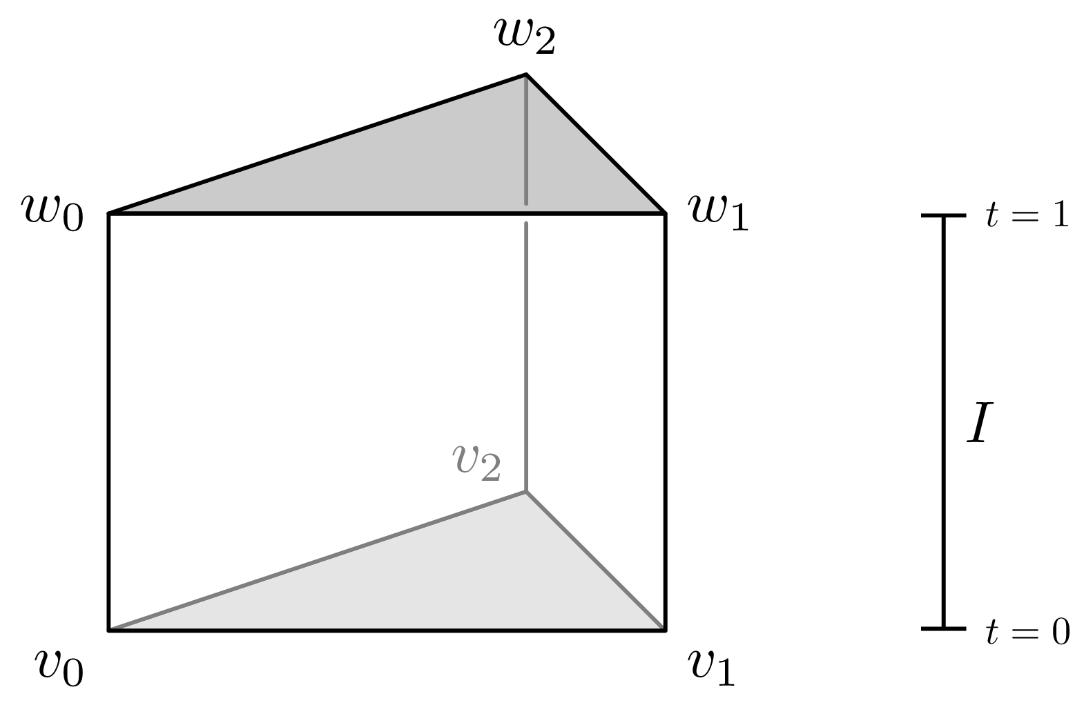
\[F:X\times I \rightarrow Y\]

and by definition, elements of \(C_n\) are continuous functions from \(\Delta^n\) to \(X\), so the composition

\[F\circ(\sigma\times\id_I):\Delta^n\times I \rightarrow Y\]

is well-defined. We first need to use this to construct an element belonging to \(C_{n+1}(Y)\). Since the domain \(\Delta^n\times I\) of this continuous function is not an \((n+1)\)-simplex, this correspondence itself does not belong to \(C_{n+1}(Y)\). Instead, we will decompose this into a sum of \((n+1)\)-simplices and use this to define a chain homotopy.

Let the vertices on the bottom face (\(t=0\)) of the domain \(\Delta^n\times I\) be \(v_0,\ldots, v_n\) and the vertices on the top face (\(t=1\)) be \(w_0,\ldots,w_n\). The case \(n=2\) is shown in the figure below.

Then we can decompose this into \((n+1)\) \((n+1)\)-simplices

\[[v_0,\ldots, v_n,w_n],\quad [v_0,\ldots, v_{n-1}, w_{n-1}, w_n],\quad\ldots,[v_0,w_0,\ldots, w_n]\]

and drawing the case \(n=2\) gives the following.

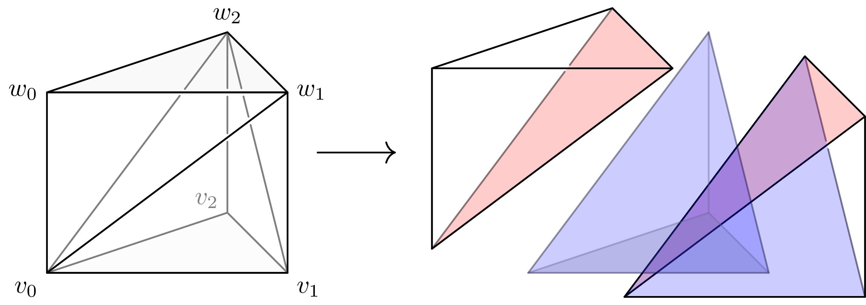
Using this decomposition, we can define

\[h_n(\sigma)=\sum_i (-1)^iF\circ(\sigma\times\id_I)\vert_{[v_0,\ldots, v_i, w_i,\ldots, w_n]}\]

and showing that this satisfies equation (1) is a simple calculation.

Therefore, homotopic continuous functions induce the same function on homology. (Homological Algebra, §Homology, ¶Proposition 6) In particular, if two spaces \(X\) and \(Y\) are homotopically equivalent and \(f:X \rightarrow Y\) and \(g:Y\rightarrow X\) are given as in Definition 4, then the homologies \(H_\bullet(X)\) and \(H_\bullet(Y)\) of the two spaces are the same.

On the other hand, from the computation in §Homology, ¶Example 8, we saw that for any space \(Y\), the singular \(k\)-complex (\(k>0\)) corresponding to a point \(y\in Y\) is always zero in \(H_k(Y)\). Therefore, if a continuous function \(f:X \rightarrow Y\) is homotopic to a constant function, then \(H_k(f)\) is the zero map for all \(k>0\). For this reason, a continuous function that is homotopic to a constant function is called null-homotopic. In particular, if the identity function \(\id_X:X \rightarrow X\) is null-homotopic, we say that \(X\) is contractible. Then by §Homology, ¶Proposition 11 and Proposition 6 above, we know that the \(k>0\)-th homology of a contractible space is always \(0\).

In the remainder of this post, we will examine homotopy equivalence and the fundamental group.

Deformation Retract

In many cases, two homotopically equivalent spaces arise as the result of a deformation called a deformation retract, and moreover, they have some geometric relationship (compared to Definition 2, which was given somewhat abruptly). To define this, we first need to define a retraction. (Set Theory, §Retraction and Section, ¶Definition 2)

Definition 7 Let \(X\) be a topological space and \(A\) be its subspace. Given the canonical inclusion \(\iota:A\rightarrow X\), if there exists a continuous function \(r:X\rightarrow A\) satisfying \(r\circ\iota=\id_A\), then \(r\) is called a (continuous) retraction onto the subspace \(A\), and in this case, \(A\) is called a retract of \(X\).

From the set-theoretic perspective, a function \(r\) satisfying the above condition always exists, but the key point is that this function \(r\) is continuous.

Example 8 For instance, it is known that for the closed disk \(D^2\) in the plane and its boundary \(S^1\), there is no retraction from \(D^2\) to \(S^1\). If a retraction \(r:D^2\rightarrow S^1\) existed, then by the functoriality of \(H_n\),

\[H_n(r)\circ H_n(\iota)=H_n(r\circ\iota)=H_n(\id_{S^1})=\id_{H_n(S^1)}\]

would hold for all \(n\). In particular, \(H_n(\iota):H_n(S^1)\rightarrow H_n(D^2)\) would have to be injective. However, in §Homology, ¶Example 8 we showed that \(H_1(D^2)\cong 0\), and by following the computation for \(D^2\setminus \left\{(0,0)\right\}\) we know that \(H_1(S^1)\neq 0\), so an injective homomorphism \(H_1(\iota)\) cannot exist.

However, comparing this example with the computation of the homology of \(D^2\setminus \left\{(0,0)\right\}\) in §Homology, ¶Example 8, we see that the nontrivial homology appearing in \(D^2\setminus \left\{(0,0)\right\}\) also appears identically in its subset \(S^1\). We know from Proposition 6 that homotopic continuous functions induce homotopic chain maps, and therefore induce the same function on homology, so how to generalize this is clear.

Definition 9 Let \(X\) be a topological space and \(A\) be its subspace, and let \(r:X\rightarrow A\) be a retraction. If there exists a homotopy \(F\) from \(\id_X\) to \(r\), then this is called a deformation retraction onto \(A\), and \(A\) is called a deformation retract of \(X\).

Then for the retraction \(r\) in Example 8 above, defining

\[t\frac{\mathbf{x}}{\lvert\mathbf{x}\rvert}+(1-t)\mathbf{x}\]

gives a homotopy from \(\id_X\) to \(r\). That is, \(S^1\) is a deformation retract of \(D^2\setminus \left\{(0,0)\right\}\).

Fundamental Group

In §Homology, ¶Example 8, we noted that if we view the \(1\)-simplex \(\Delta^1\) as \(I=[0,1]\), then the elements generating \(C_1(X)\) can be thought of as paths on \(X\) by definition, and when we obtain the homology \(H_1(X)\), we consider closed paths. This is essentially the same as looking at functions from \(S^1\) to \(X\). Let us examine this more rigorously.

First, for two homotopic continuous functions \(f,g:X \rightarrow Y\) and a homotopy \(F\) between them, if for a subset \(A\subseteq X\) the equation

\[F(x,t)=f(x)\qquad\text{for all $t\in[0,1]$}\]

holds, then \(F\) is called a homotopy relative to \(A\). If in Definition 9, the homotopy \(F\) is a homotopy relative to \(A\), then we say that \(A\) is a strong deformation retract of \(X\).

Now for any two paths \(\alpha_0,\alpha_1:I\rightarrow X\), a path homotopy between them means a homotopy relative to \(\{0,1\}\). That is, two paths \(\alpha_0,\alpha_1\) share their endpoints (i.e., \(\alpha_0(0)=\alpha_1(0)\) and \(\alpha_0(1)=\alpha_1(1)\)) and the homotopy \((\alpha_t)_{0\leq t\leq 1}\) preserves the endpoints so that

\[\alpha_0(0)=\alpha_t(0)=\alpha_1(0),\qquad \alpha_0(1)=\alpha_t(1)=\alpha_1(1)\qquad\text{for all $0\leq t \leq 1$}\]

holds.

Definition 10 If there exists a path homotopy between two paths \(\alpha_0,\alpha_1:I\rightarrow X\), we say they are path homotopic and write \(\alpha_0\sim \alpha_1\).

Then, by slightly adapting the proof of Proposition 3, we know that path homotopy gives an equivalence relation on the set of paths with endpoints \(p\) and \(q\). Moreover, it is clear that this equivalence relation preserves reparametrization: for any path \(\alpha:I \rightarrow X\) and any reparametrization \(\varphi:I\rightarrow I\) (i.e., a homeomorphism preserving \(0\) and \(1\)), defining

\[\alpha_t(s)=\alpha(t\varphi(s)+(1-t)s)\]

gives a path homotopy between \(\alpha_0=\alpha\) and \(\alpha_1=\alpha\circ\varphi\). Using this, we define the product of two paths by the equation

\[(\alpha\ast \beta)(s)=\begin{cases}\alpha(2s)&0\leq s \leq 1/2\\ \beta(2s-1)&1/2\leq s \leq 1\end{cases}\tag{$\ast\ast$}\]

For this to be a continuous path, of course, we need \(\alpha(1)=\beta(0)\). Then the following properties hold.

1. If \(\alpha_0\sim \alpha_1\) and \(\beta_0\sim \beta_1\) and \(\alpha_0\ast \beta_0\) is well-defined, then \(\alpha_1\ast \beta_1\) is also well-defined and \(\alpha_0\ast \beta_0\sim \alpha_1\ast \beta_1\) holds. This is clear by considering the homotopy \(\alpha_t\ast \beta_t\).
2. Therefore, if we give \(C(I,X)\) the equivalence relation of path homotopy, then through the equation \([\alpha]\ast[\beta]=[\alpha\ast \beta]\), for each \(\alpha,\beta\) satisfying \(\alpha(1)=\beta(0)\), the operation on \([\alpha]\) and \([\beta]\) is well-defined.
3. Then for the constant paths \(c_{\alpha(0)}\) and \(c_{\alpha(1)}\) staying at the points \(\alpha(0)\) and \(\alpha(1)\) respectively, we have \([c_{\alpha(0)}]\ast [\alpha]=[\alpha]=[\alpha]\ast[c_{\alpha(1)}]\). This is because, roughly speaking, path homotopy preserves reparametrization, so in equation (\(\ast\ast\)) we can replace \(1/2\) with any number between \(0\) and \(1\), and approaching this number to \(0\) or \(1\) gives the desired homotopy. By almost the same argument, we can show that \(\ast\) is associative.
4. Moreover, inverses exist: for any path \(\alpha\), defining \(\bar{\alpha}(t)=\alpha(1-t)\) gives \([\alpha]\ast[\bar{\alpha}]=[c_{\alpha(0)}]\) and \([\bar{\alpha}]\ast[\alpha]=[c_{\alpha(1)}]\).

Summarizing these results, we have the following.

Definition 11 By the above results, \(C(I,X)/{\sim}\) forms a groupoid, which is called the fundamental groupoid of \(X\) and denoted by \(\Pi_1(X)\). (Category Theory, §Categories, ¶Definition 11)

That is, for any space \(X\), the fundamental groupoid \(\Pi_1(X)\) is a category whose objects are the points of \(X\), and whose morphisms between two points \(x\) and \(y\) are the homotopy types of paths from \(x\) to \(y\). As a full subcategory of \(\Cat\), a morphism in \(\Grpd\) is simply a functor. Explicitly, given any continuous map \(f:X \rightarrow Y\), \(\Pi_1(f):\Pi_1(X)\rightarrow\Pi_1(Y)\) is defined on objects by \(x\mapsto f(x)\) and on morphisms by the composition

\[\Pi_1(f)([\alpha])=[f\circ\alpha]\]

and that this is well-defined is clear since for two paths \(\alpha_0\sim\alpha_1\), if \(\alpha_t\) is a path homotopy between them, then \(f\circ \alpha_t\) is a path homotopy between \(f\circ\alpha_0\) and \(f\circ\alpha_1\). Moreover, if two continuous maps \(f_0,f_1:X \rightarrow Y\) are homotopic, then there exists a natural isomorphism between the two functors \(\Pi_1(f_0)\) and \(\Pi_1(f_1)\) they induce. (Category Theory, §Natural Transformations, ¶Definition 1) That is, for any path \(\alpha:I \rightarrow X\) with starting point \(x_0\) and endpoint \(x_1\), the following diagram

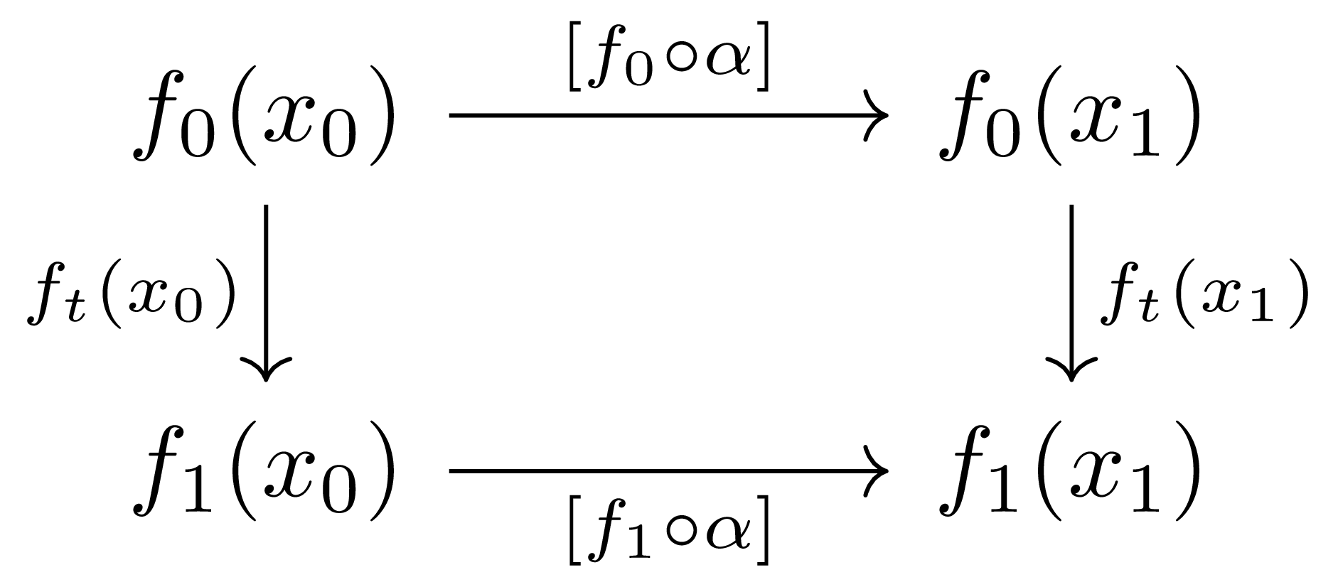
commutes (up to path homotopy). Here \(f_t(x_0)\) and \(f_t(x_1)\) are the paths arising from the homotopy \((f_t)_{0\leq t\leq 1}\), and commutativity is clear from the path homotopy

\[F(s,t)=f_t(\alpha(s))\]

In particular, if we consider only paths with a fixed point \(x\in X\) as both starting point and endpoint (i.e., loops with \(x\) as the base point), this is the same as considering the endomorphism monoid at \(x\) in the category \(\Pi_1(X)\), and since \(\Pi_1(X)\) is a groupoid, this is in fact an automorphism group. We write this as

\[\pi_1(X,x)=\Aut_{\Pi_1(X)}(x)\]

and if \(X\) is path-connected, this group does not depend on the choice of \(x\). This is called the fundamental group of \(X\), and it is the skeleton of \(\Pi_1(X)\). (Category Theory, §Natural Transformations, ¶Definition 4) Therefore, \(\pi_1(X,x)\) is equivalent to \(\Pi_1(X)\) as a category. As we saw above, homotopic continuous functions induce natural isomorphisms between fundamental groupoids, so we know that the fundamental groupoid and fundamental group are homotopy invariants.

Example 12 For example, the fundamental groupoid \(\Pi_1(\mathbb{R^n})\) of the space \(\mathbb{R}^n\) is a category consisting of the following data.

• The objects of \(\Pi_1(\mathbb{R}^n)\) are exactly the points of \(\mathbb{R}^n\).

• For any \(\mathrm{x}_1,\mathrm{x}_2\in \mathbb{R}^n\), there exists a unique morphism from \(\mathrm{x}_1\) to \(\mathrm{x}_2\). That is, any path \(\alpha_1:I \rightarrow \mathbb{R}^n\) starting at \(\mathrm{x}_1\) and going to \(\mathrm{x}_2\) is always path homotopic to the following path

  \[\alpha_0:t\mapsto (1-t)\mathrm{x}_1+t\mathrm{x}_2\]

  This can be easily verified by setting \(\alpha_t=(1-t)\alpha_1+t\alpha_0\).

Therefore, for any \(\mathrm{x}\), \(\pi_1(\mathbb{R},\mathrm{x})\) is the trivial group.

---

References

[Hat] A. Hatcher, Algebraic Topology. Cambridge University Press, 2022.
[Mun] James Munkres, Topology. Prentice Hall, 2000.

---