
This post was translated from Korean by LLM (Kimi). The translation may contain errors or awkward sentences. The Korean original is the source of truth.
Vector Bundles
Now we need to define vector fields, but in order to define notions such as $C^\infty$ vector fields it is better to first define the concept of a vector bundle. Let us first define a vector bundle over a topological space.
Definition 1 A vector bundle over a topological space $B$ is an object $\pi:E \rightarrow B$ defined as follows.
- The total space $E$ and the base space $B$ are both topological spaces, and $\pi:E \rightarrow B$ is a continuous surjection.
- For each $b\in B$, the fiber $E_b=\pi^{-1}(b)$ carries the structure of a $k$-dimensional vector space.
- For each $b_0\in B$ there exist a suitable open neighborhood $U\subseteq B$ and a homeomorphism $h:U\times\mathbb{R}^k \rightarrow\pi^{-1}(U)$ such that for every $b\in U$, the map $x\mapsto h(b,x)$ is an isomorphism.
We call $k$ the rank of the vector bundle $E\rightarrow B$. We call the homomorphism $h$ in the third condition a local trivialization, and if we can take $U=B$, we call $E$ a trivial vector bundle.
Similarly, we can define a vector bundle over a manifold. To do this, we change both $E$ and $B$ to manifolds, change $\pi$ to a $C^\infty$ surjection, and replace the third condition with
For each $b_0\in B$ there exist a suitable coordinate system $U\subseteq B$ and a diffeomorphism $h:U\times\mathbb{R}^k\rightarrow\pi^{-1}(U)$ such that for every $b\in U$, the map $x\mapsto h(b,x)$ is an isomorphism.
Tangent Bundles
A typical example of a vector bundle is the tangent bundle.
Example 2 (Tangent bundle) Define the set $TM$ by
\[TM=\bigsqcup_{p\in M} T_pM\]Then there is a natural projection map $\pi:TM\rightarrow M$. To regard $TM$ as a vector bundle we must endow it with a manifold structure.
First, let us define a coordinate system on $TM$. For an arbitrary coordinate system $(U,\varphi)$, define a function $\tilde{\varphi}:\pi^{-1}(U)\rightarrow\mathbb{R}^m\times\mathbb{R}^m$ by the formula
\[\tilde{\varphi}(v)=\bigl(x^1(\pi(v)), \ldots, x^m(\pi(v)), dx^1(v),\ldots, dx^m(v)\bigr)\]Then $\tilde{\varphi}$ is a bijection from $\pi^{-1}(U)$ onto the open subset $\varphi(U)\times\mathbb{R}^m$ of $\mathbb{R}^{2m}$.
These are $C^\infty$-compatible. Given another coordinate system $(V,\psi)$, $\psi=(y^j)_{j=1}^m$, define $\tilde{\psi}$ as above. Then on $\pi^{-1}(U)\cap\pi^{-1}(V)=\pi^{-1}(U\cap V)$ we have
\[\begin{aligned}(\tilde{\psi}\circ\tilde{\varphi}^{-1})(p^1, \ldots, p^m, v^1, \ldots, v^m)&=\tilde{\psi}\left(\varphi^{-1}(p), \sum v^i\frac{\partial}{\partial x^i}\bigg|_{\varphi^{-1}(p)}\right)\end{aligned}\]Here, letting $v=\sum v^i\frac{\partial}{\partial x^i}$, the right-hand side can simply be written as
\[\left((\psi\circ\varphi^{-1})(p), dy^1(v), \ldots, dy^m(v)\right)\]Now for arbitrary $j$ we have
\[dy^j\left(\sum v^i\frac{\partial}{\partial x^i}\bigg|_{\varphi^{-1}(p)}\right)=\sum_{i=1}^m v^i\frac{\partial y^j}{\partial x^i}\bigg|_{\varphi^{-1}(p)}\]Therefore, since each component of the transition map $\tilde{\psi}\circ\tilde{\varphi}^{-1}$ above is $C^\infty$, the map $\tilde{\psi}\circ\tilde{\varphi}^{-1}$ is also $C^\infty$.
Meanwhile, the topology on $TM$ is obtained by taking the collection
\[\{\tilde{\varphi}^{-1}(W)\mid \text{$W$ open in $\mathbb{R}^{2m}$, $(U,\varphi)\in\mathcal{A}$}\}\]as a basis. Taking $W=\mathbb{R}^{m}$, one can check that the $\pi^{-1}(U)$ are all open in the topology generated by the above sets, and one can also verify that this topology yields a $2m$-dimensional topological manifold.
All that remains is the local trivialization on $TM$. For an arbitrary coordinate system $(U,\varphi)$, define $\phi:\pi^{-1}(U)\rightarrow U\times\mathbb{R}^m$ this time by the formula
\[v|_p\mapsto (p, dx^1(v),\ldots, dx^m(v))\]That is all that is needed. That $\phi$ is a vector-space isomorphism on each fixed $\pi^{-1}(p)$ is obvious, and it is also obvious that $(\pi\circ\phi)(x,v)=x$ for any $v_x$. That $\phi$ is a diffeomorphism follows from
\[\tilde{\varphi}=(\varphi\times\id_{\mathbb{R}^m})\circ\phi\]and the fact that the two functions other than $\phi$ in this formula are both diffeomorphisms.
In particular, if $TM$ is a trivial bundle, we call $M$ a parallelizable manifold.
Smooth Functors
The reason the tangent bundle $TM$ is important is that most vector bundles defined over a manifold are defined from $TM$. For example, the cotangent bundle $T^\ast M$ is the vector bundle with the cotangent space $T_p^\ast M$, the dual space of the tangent space, attached at each $p\in M$. Similarly, various vector bundles are defined by applying operations from linear algebra (Example 5) at each point $p$.
Ordinarily, whenever we define these we would have to verify that they satisfy the conditions of a vector bundle, but [Mil] presents a more fundamental approach.
Definition 3 Let two vector bundles $E\rightarrow B$, $E’\rightarrow B’$ be given. Then a bundle map from $E \rightarrow B$ to $E’ \rightarrow B’$ is, among pairs $E\rightarrow E’, B \rightarrow B’$ making the diagram
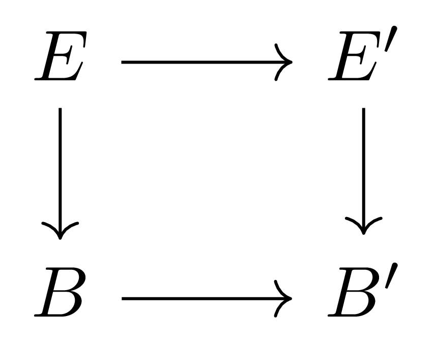
commute, one for which $E_b\rightarrow E’_{b’}$ is an isomorphism.
Now consider the category $\mathbf{FVect}\text{iso}$ of finite-dimensional $\mathbb{R}$-vector spaces whose morphisms are isomorphisms. Then $\mathbf{FVect}\text{iso}\times\mathbf{FVect}_\text{iso}$ is the category whose
- objects are pairs $(V,W)$ of finite-dimensional vector spaces,
- morphisms are pairs $(V,W)\overset{(f,g)}{\longrightarrow}(V’,W’)$ of isomorphisms between finite-dimensional vector spaces.
Hence a functor $F$ from $\mathbf{FVect}\text{iso}\times\mathbf{FVect}\text{iso}$ to $\mathbf{FVect}_\text{iso}$ must take $(V,W)$ to an $\mathbb{R}$-vector space $F(V,W)$ and $(f,g)$ to an isomorphism $F(f,g)$.
Definition 4 A functor $F:\mathbf{FVect}\text{iso}\times\mathbf{FVect}\text{iso}\rightarrow \mathbf{FVect}_\text{iso}$ is called a smooth functor if $F(f,g)$ depends smoothly on $f,g$.
If $f\in\Hom(V,V’), g\in\Hom(W,W’)$, then $F(f,g)\in\Hom(F(V,W),F(V’,W’))$. Since these are all vector spaces, they carry differential structures as in §Examples of Manifolds, ⁋Example 2, and through this the above definition can be applied. Also, it is not difficult to extend this definition to a general $k$-fold product
\[\mathbf{FVect}_\text{iso}\times\cdots\times\mathbf{FVect}_\text{iso}\rightarrow \mathbf{FVect}_\text{iso}\]Example 5 $\Hom(-,-)$ is a smooth functor. Let two isomorphisms $f:V\rightarrow V’$, $g:W\rightarrow W’$ be given. Then $\Hom(f,g)$ is a functor from $\Hom(V,W)$ to $\Hom(V’,W’)$ and makes the diagram below
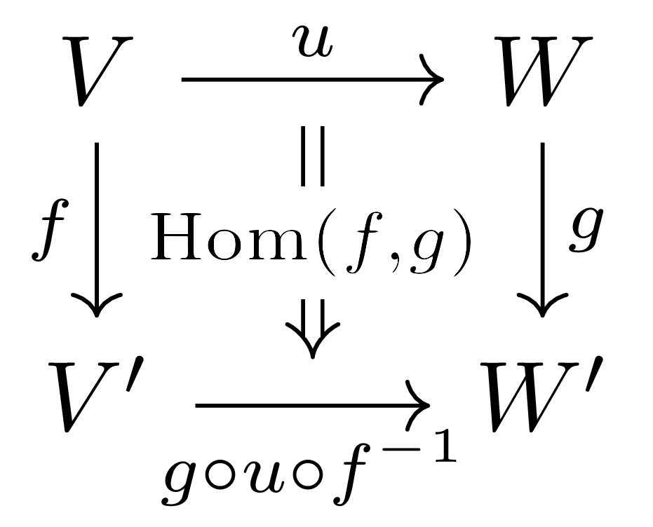
commute. Writing this as a formula, we can say $\Hom(f,g)(u)=g\circ u\circ f^{-1}$. That $\Hom(f,g)$ depends smoothly on $g$ can be easily verified. Consider the correspondence $g\mapsto \Hom(f,g)$. Then for a basis $w_i^j$ of $\Hom(W,W’)$,
\[(g+tw_i^j)\circ u\circ f^{-1}=g\circ u\circ f^{-1}+tw_i^j\circ u\circ f^{-1}\]holds for all $u$, so the directional derivative of this correspondence in the $w_i^j$-direction is $u\mapsto w_i^j\circ u\circ f^{-1}$, which is continuous. Moreover, this argument remains valid no matter what linear map is substituted in place of $g$, so from this we know that arbitrary higher-order directional derivatives of $g\mapsto\Hom(f,g)$ are always continuous. That is, $g\mapsto\Hom(f,g)$ is $C^\infty$. That this correspondence also depends smoothly on $f$ is somewhat more tedious than for $g$, but because $f$ is an isomorphism we can choose $t$ sufficiently small so that $f+tw_i^j$ is invertible, and then repeat the argument above.
The following are all examples of smooth functors.
- Dual functor $(-)^\ast$ ([Linear Algebra] §Dual Space),
- $k$-th tensor functor $\mathcal{T}^k(-)$ ([Multilinear Algebra] §Tensor Algebras),
- $k$-th symmetric functor $\mathcal{S}^k(-)$ ([Multilinear Algebra] §Tensor Algebras),
- $k$-th exterior functor $\bigwedge\nolimits^k(-)$ ([Multilinear Algebra] §Tensor Algebras),
- Tensor product $-\otimes -$,
- Direct sum $-\oplus-$.
The proof of the following theorem can be found in Theorem 3.6 of [MS].
Theorem 6 Let an arbitrary smooth functor $F:(\mathbf{FVect}\text{iso})^n\rightarrow \mathbf{FVect}\text{iso}$ and $n$ vector bundles $E_i\rightarrow B$ with a common base space $B$ be given. Then there exists a vector bundle $E\rightarrow B$ whose fiber at each $b\in B$ is given by
\[E_b=F((E_1)_b,\ldots,(E_n)_b)\]The vector bundle $E$ obtained by the above process is simply denoted by $F(E_1,\ldots, E_n)$.
Cotangent Bundles
Applying Theorem 6 above to an arbitrary manifold $M$, the tangent bundle $E=TM\rightarrow M$, and the dual functor $(-)^\ast$, we obtain the following.
Definition 7 The cotangent bundle over a manifold $M$ means the vector bundle $(TM)^\ast$ obtained by Theorem 6. In keeping with the notation $T_p^\ast M$ for the cotangent space, we denote this by $T^\ast M$.
$T^\ast M$ is the space with the vector space $T_p^\ast M$ attached at each point $p$. Here $T_p^\ast M$ is the dual space of the vector space $T_pM$, that is, the space of linear maps that take a vector of $T_pM$ and output a real number. We will revisit vector bundles obtained by applying other smooth functors before long.
References
[MS] J.W. Milnor and J.D. Stasheff, Characteristic classes, Princeton university press, 1974.
댓글남기기