
This post was translated from Korean by LLM (Kimi). The translation may contain errors or awkward sentences. The Korean original is the source of truth.
In the previous post we saw two different ways of giving a manifold structure on \(\mathbb{R}\). In this post we examine various examples of topological spaces equipped with manifold structures.
Since a manifold is a structure that locally resembles \(\mathbb{R}^m\), the simplest example is of course \(\mathbb{R}^m\) itself.
Example 1 The standard differentiable structure on \(\mathbb{R}^m\) with the standard topology is given by the atlas \(\{(\mathbb{R}^m,\id_{\mathbb{R}^m})\}\).
As in the examples from the previous post, it is also possible to give different differentiable structures on \(\mathbb{R}^m\).
Example 2 More generally, let \(V\) be an \(m\)-dimensional \(\mathbb{R}\)-vector space. Choose a basis \(\mathcal{B}\) of \(V\), and consider the coordinate representation \(\varphi_\mathcal{B}:v\mapsto [v]_{\mathcal{B}}\) with respect to \(\mathcal{B}\). This linear map is an isomorphism, hence a bijection, and therefore we can transfer both the topology and the differentiable structure of \(\mathbb{R}^m\) to \(V\) via it. Transferring the differentiable structure of \(\mathbb{R}^m\) to \(V\) via \(\varphi_\mathcal{B}\) is the same as defining a differentiable structure on \((V,\mathcal{B})\) through a single coordinate system \((V,\varphi_{\mathcal{B}})\).
Of course, these functions themselves depend on the choice of basis, but the topology and differentiable structure defined in this way are independent of the choice of basis.
First, a norm on \(V\) defined in this manner gives an equivalent metric structure regardless of the choice of basis, so the vector spaces \((V,\mathcal{B})\) and \((V,\mathcal{C})\) with different bases \(\mathcal{B}\) and \(\mathcal{C}\) have the same topological structure. Moreover, they also have the same differentiable structure. To see this, it suffices to show that the transition maps \(\varphi_\mathcal{B}\circ\varphi_\mathcal{C}^{-1}\) and \(\varphi_\mathcal{C}\circ\varphi_\mathcal{B}^{-1}\) for \((V,\varphi_\mathcal{B})\) and \((V,\varphi_\mathcal{C})\) are both \(C^\infty\); but these are in fact matrices, and hence polynomials, so they are obviously \(C^\infty\).
As special cases of this,
- The set \(\Mat_n(\mathbb{R})\) of \(n\times n\) matrices is an \(n^2\)-dimensional vector space, so it has a differentiable structure.
- \(\mathbb{C}^n\) can be regarded as a \(2n\)-dimensional \(\mathbb{R}\)-vector space, so it also has a differentiable structure.
To give further examples, we first need to define the following.
Definition 3 Let \(M\) be a manifold. Give an open subset \(V\) of \(M\) the following two structures
- the subspace topology inherited from the topology of \(M\),
-
for the differentiable structure \(\mathcal{A}\) defined on \(M\),
\[\mathcal{A}_V=\{(U_\alpha\cap V,\varphi_\alpha|_{U_\alpha\cap V})\mid(U_\alpha,\varphi_\alpha)\in\mathcal{A}\}\]
then \(V\) becomes a manifold of the same dimension as \(M\). We call such a manifold structure an open submanifold of \(M\).
Of course, for this definition to be well defined, the subspace topology must satisfy the locally Euclidean, second countable, and Hausdorff conditions, and the elements of \(\mathcal{A}_V\) must be pairwise \(C^\infty\)-compatible. However, the Hausdorff and second countability properties are both preserved under the subspace topology, and the locally Euclidean property also follows from the fact that \(V\) is an open set. Moreover, the transition maps between elements of \(\mathcal{A}_V\) are restrictions of \(C^\infty\) functions, so they are also \(C^\infty\).
Example 4 Among the elements of \(\Mat_{n}(\mathbb{R})\), the set \(\GL(n,\mathbb{R})\) of invertible \(n\times n\) matrices is the collection of matrices satisfying \(\det(A)\neq 0\). Regarding the determinant \(\det\) as a function from \(\Mat_n(\mathbb{R})\) to \(\mathbb{R}\), this function is a polynomial, hence continuous, and therefore \(\GL(n,\mathbb{R})\), being the preimage of the open set \(\mathbb{R}\setminus\{0\}\), is also an open subset of \(\Mat_n(\mathbb{R})\). Thus \(\GL(n,\mathbb{R})\) is an \(n^2\)-dimensional manifold.
On the other hand, \(\GL(n,\mathbb{R})\) is the disjoint union of the matrices with \(\det A>0\) and those with \(\det A<0\), and each of these sets is open for the same reason as above, so \(\GL(n,\mathbb{R})\) is not connected.
Example 5 For an open set \(U\subset\mathbb{R}^m\) and a \(C^\infty\) function \(f:U\rightarrow\mathbb{R}^n\), define the graph \(\graph(f)\) of \(f\) to be the following set
\[\graph(f)=\{(x,y)\in\mathbb{R}^m\times\mathbb{R}^n\mid \text{$x\in U$, $y=f(x)$}\}\]Then \(f:U\rightarrow\graph(f)\) and the projection \(\pr:\graph(f)\rightarrow U\) onto the first \(m\) coordinates are both continuous and are inverses of each other, so \(\graph(f)\) and \(U\) are homeomorphic. Therefore \(\graph(f)\) is a topological manifold, and in particular the projection \(\pr:\graph(f)\rightarrow U\) forms an atlas consisting of a single chart \(\{(\graph(f),\pr)\}\), so it also carries a natural (differentiable) manifold structure.
In all the examples so far we have given the differentiable structure via an atlas consisting of a single chart, which means that the manifold resembles \(\mathbb{R}^m\) not only locally but also globally, so this is not a very interesting situation.
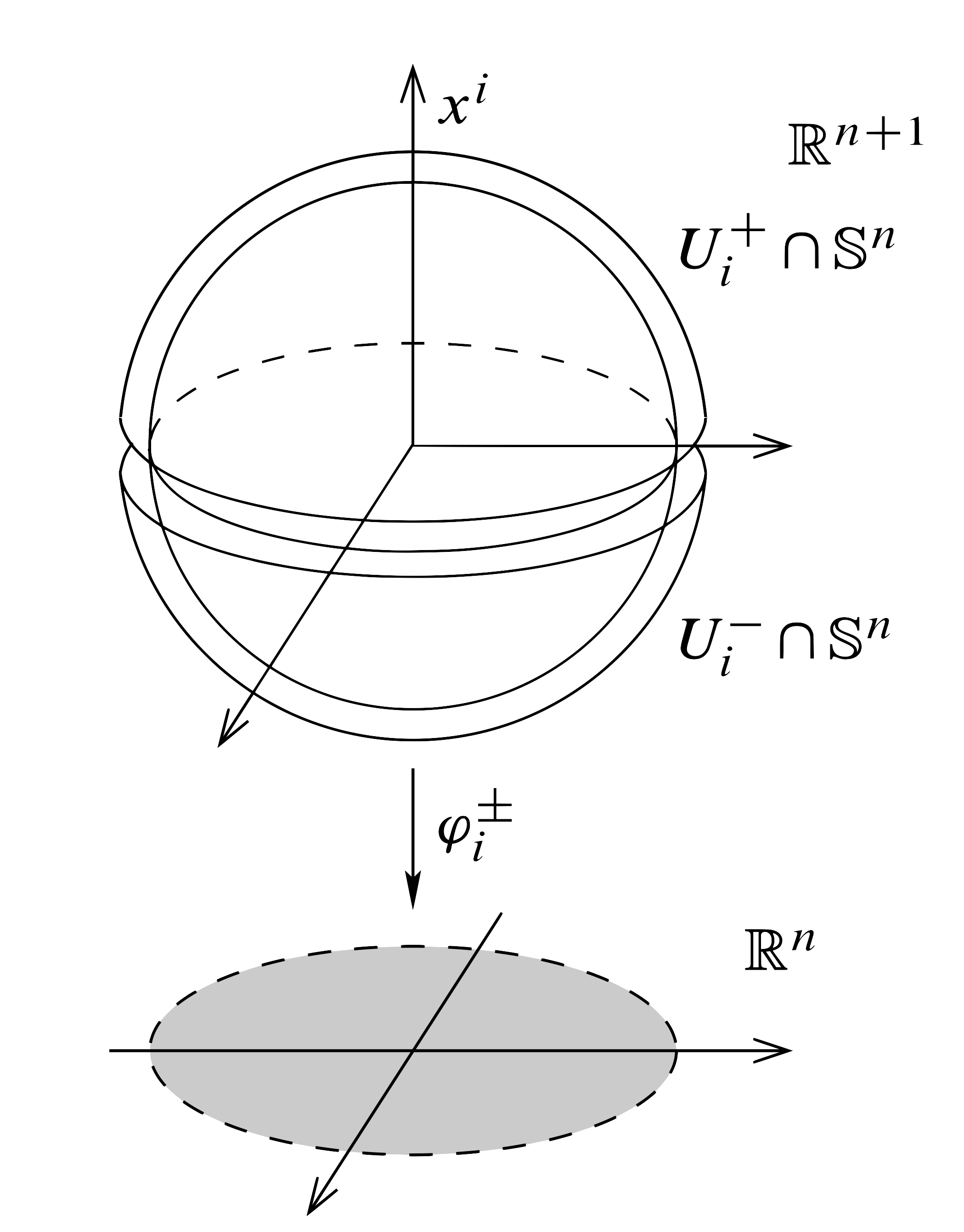
Example 6 Consider the \(n\)-dimensional sphere \(S^n\) in \(\mathbb{R}^{n+1}\). If we give \(S^n\) the subspace topology, the Hausdorff and second countability conditions are both satisfied. However, since \(S^n\) is not an open set, showing the locally Euclidean condition is more difficult than in the case of an open submanifold.
Pick any \(p\in S^n\). Since \(0\not\in S^n\), some coordinate of \(p\) must be nonzero. Without loss of generality, let this coordinate be the \((n+1)\)-st coordinate, and assume it is positive. That is, \(p\) belongs to the set
\[U_{n+1}^+=\{(x^1, x^2, \ldots, x^{n+1})\in\mathbb{R}^{n+1}\mid x^{n+1}>0\}\]From the picture it is almost obvious that \(U_{n+1}^+\) and \(D^n\) are homeomorphic.
To write this down rigorously with formulas, define a function \(f:D^n\rightarrow\mathbb{R}\) for each point \(x=(x^1,\ldots, x^n)\) in \(D^n\) by the formula
\[f(x)=\sqrt{1-\lvert x\rvert^2}\]Then \(f\) is \(C^\infty\) on \(D^n\), and moreover it defines a homeomorphism between \(D^n\) and \(\graph(f)=U_{n+1}^+\). Therefore the locally Euclidean condition holds.
Furthermore, the following collection of these \(U_i^\pm\) and the projections \(\varphi_i^\pm\) onto the \(n\) coordinates omitting the \(i\)-th coordinate
\[\mathcal{A}=\{(U_i^\pm, \varphi_i^\pm\mid i=1,2,\ldots, n+1\}\]forms an atlas. To verify this, we must show that the charts constituting this atlas are pairwise \(C^\infty\)-compatible. \(U_i^+\) and \(U_i^-\) do not meet, so they are trivially \(C^\infty\)-compatible with each other. Let two charts \((U_i^\pm, \varphi_i^\pm)\) and \((U_j^\pm,\varphi_j^\pm)\) with distinct indices \(i,j\) be given. Then first, under \((\varphi_i^\pm)^{-1}\),
\[(x^1, x^2, \ldots, x^n)\mapsto (x^1, x^2, \ldots, x^{i-1}, \pm \sqrt{1-\lvert x\rvert^2}, x^i, \ldots, x^n)\]and subsequently under \(\varphi_j^\pm\),
\[(x^1, x^2, \ldots, x^{i-1}, \pm \sqrt{1-\lvert x\rvert^2}, x^i, \ldots, x^n)\mapsto (x^1, x^2, \ldots, \hat{x}^j, \ldots, x^{i-1}, \pm \sqrt{1-\lvert x\rvert^2}, x^i, \ldots, x^n)\]Here \(\hat{x}^j\) means that the \(j\)-th component is omitted. In this case, since each component of the right-hand side is a \(C^\infty\) function of the \(x^i\)’s, the composition \((\varphi_j^{\pm})\circ(\varphi_i^\pm)^{-1}\) is \(C^\infty\), and similarly one can check that \((\varphi_i^{\pm})\circ(\varphi_j^\pm)^{-1}\) is also \(C^\infty\). Therefore the above collection \(\mathcal{A}\) defines a differentiable structure on \(S^n\).
The differentiable structure defined on \(S^n\) is a typical example of a manifold. The next example gives the (same) differentiable structure on \(S^n\) by a method different from the above, using the differential, and this example can be further generalized to give a manifold structure.
Example 7 Let \(U\) be a subset of \(\mathbb{R}^n\) and let \(F\) be a \(C^\infty\) function defined on \(U\). Then the level set \(M=F^{-1}(c)\) is well defined. If in addition the following Jacobian matrix
\[\begin{pmatrix}\frac{\partial F^1}{\partial x^1}&\frac{\partial F^1}{\partial x^2}&\cdots&\frac{\partial F^1}{\partial x^n}\\\frac{\partial F^2}{\partial x^1}&\frac{\partial F^2}{\partial x^2}&\cdots&\frac{\partial F^2}{\partial x^n}\\\vdots&\vdots&\ddots&\vdots\\\frac{\partial F^n}{\partial x^1}&\frac{\partial F^n}{\partial x^2}&\cdots&\frac{\partial F^n}{\partial x^n}\end{pmatrix}\]is never zero; that is, for each point \(a\in M\) there exists some \(i\) such that the column vector \(dF/dx^i\) is not the zero vector. Then by the implicit function theorem, in a suitable open neighborhood of the point \(a\), \(M\) is the graph of a function \(f\) of the form
\[x^i=f(x^1,\ldots, \hat{x}^i,\ldots, x^n)\]Now, just as in Example 6, if we give \(M\) the subspace topology and construct charts using the \((U, f)\) just made, we can verify that \(M\) becomes an \((n-1)\)-dimensional manifold.
Using Example 7, we can regard \(S^n\) as the zero set of the function
\[F(x^1,\ldots, x^{n+1})=(x^1)^2+(x^2)^2+\cdots+(x^{n+1})^2-1\]defined on \(\mathbb{R}^{n+1}\); hence Example 6 can be seen as a special case of the above example.
Example 8 Suppose a relation on the set \(\mathbb{R}^{n+1}\setminus\{0\}\) is defined by \(x\sim y\iff \exists\lambda(x=\lambda y)\). It is not hard to check that \(\sim\) is an equivalence relation. Now consider the quotient set \(\RP^n=\RP^n/\sim\) with the quotient topology defined via the canonical projection \(\pi:\mathbb{R}^{n+1}\setminus\{0\}\rightarrow \RP^n\), and let \([x]\) be the representative of \(x\in\mathbb{R}^{n+1}\setminus\{0\}\).
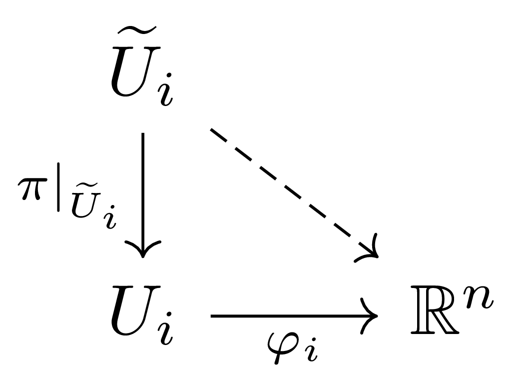
For each \(i=1,\ldots, n+1\), consider the open subset
\[\tilde{U}_i=\{(x^1,\ldots, x^{n+1})\mid x^i\neq 0\}\]of \(\mathbb{R}^{n+1}\setminus\{0\}\). Then \(\tilde{U}_i\) is a saturated open set, so by [Topology] §Quotient Spaces, ⁋Proposition 8 the quotient map \(\pi\) restricts well to \(\tilde{U}_i\). Therefore, if we define the function \(\varphi_i:U_i\rightarrow\mathbb{R}^n\) by
\[\varphi_i[x^1,\ldots, x^{n+1}]=\left(\frac{x^1}{x^i},\ldots,\frac{x^{i-1}}{x^i},\frac{x^{i+1}}{x^i},\ldots, \frac{x^{n+1}}{x^i}\right)\]1 the function \(\varphi_i\circ\pi\vert_{\tilde{U}_i}\) is continuous, and hence by [Topology] §Quotient Spaces, ⁋Proposition 9 \(\varphi_i\) is also continuous.
Moreover, the following continuous function
\[\psi_i:(u^1, \ldots, u^n)\mapsto [u^1, \ldots, u^{i-1}, 1, u^i,\ldots, u^n]\]is easily seen to be the inverse of \(\varphi_i\), so these \(U_i\) are all homeomorphic to \(\mathbb{R}^n\). That is, \(\RP^n\) is \(n\)-dimensional locally Euclidean. Since the quotient topology makes \(\RP^n\) Hausdorff and second countable, \(\RP^n\) becomes a topological manifold.
On the other hand, considering the transition maps between these \((U_i,\varphi_i)\) and \((U_j,\varphi_j)\), first under \(\varphi_j^{-1}\),
\[(u^1, \ldots, u^n)\mapsto [u^1, \ldots, u^{j-1}, 1, u^j,\ldots, u^n]\]and then applying \(\varphi_i\),
\[[u^1, \ldots, u^{j-1}, 1, u^j,\ldots, u^n]\mapsto \left(\frac{u^1}{u^i},\ldots,\frac{u^{j-1}}{u^i}, \frac{1}{u^i}, \frac{u^j}{u^i},\ldots, \frac{u^{i-1}}{u^i},\frac{u^{i+1}}{u^i},\ldots, \frac{u^{n+1}}{u^i}\right)\]so they are \(C^\infty\)-compatible.
Finally, let us look at a slightly more general example.
Example 9 Let \((M,\mathcal{A}_M)\) and \((N,\mathcal{A}_N)\) be manifolds of dimensions \(m\) and \(n\), respectively. Then their product manifold is the manifold obtained by giving \(M\times N\) the product topology and defining the differentiable structure by
\[\mathcal{A}=\{(U_\alpha\times V_\beta,\varphi_\alpha\times\psi_\beta)\mid (U_\alpha,\varphi_\alpha)\in\mathcal{A}_M,(V_\beta,\psi_\beta)\in\mathcal{A}_N\}\]References
[Lee] John M. Lee. Introduction to Smooth Manifolds, Graduate texts in mathematics, Springer, 2012
[War] Frank W. Warner. Foundations of Differentiable Manifolds and Lie Groups, Graduate texts in mathematics, Springer, 2013
-
In fact, since this function is a map from a subset of \(\RP^n\) to \(\mathbb{R}^n\), we must show that the right-hand side does not depend on the choice of representative. That is, even if we choose \([\lambda x^1,\ldots, \lambda x^{n+1}]\) as the representative, the same result must come out, and this is clear from the formula. ↩
댓글남기기