
This post was translated from Korean by LLM (Kimi). The translation may contain errors or awkward sentences. The Korean original is the source of truth.
In the previous post, we saw that for two $\mathbb{K}$-vector spaces $V,W$ of dimensions $n$ and $m$ respectively, $\Hom(V,W)$ is an $mn$-dimensional $\mathbb{K}$-vector space. Also, the space $\Mat_{m\times n}(\mathbb{K})$ of $m\times n$ matrices is an $mn$-dimensional $\mathbb{K}$-vector space. Thus, from §Isomorphic Vector Spaces, ⁋Corollary 4 we know that these two vector spaces are isomorphic.
The fundamental theorem of linear algebra1 that we will prove in this post shows not only that they are isomorphic simply because they are vector spaces of the same dimension, but that there exists a natural isomorphism between them, proving that these two are essentially the same space.
Fundamental Theorem: Euclidean Space
In §The Space of Linear Maps we understood a linear map $L$ satisfying the following equations
\[\begin{aligned}L(x_1)&=\alpha_{11}y_1+\alpha_{21}y_2+\cdots+\alpha_{m1}y_m\\L(x_2)&=\alpha_{12}y_1+\alpha_{22}y_2+\cdots+\alpha_{m2}y_m\\&\phantom{a}\vdots\\L(x_n)&=\alpha_{1n}y_1+\alpha_{2n}y_2+\cdots+\alpha_{mn}y_m\end{aligned}\]via the correspondence
\[v=\sum_{i=1}^n v_ix_i\quad\mapsto\quad \sum_{j=1}^m\left(\sum_{i=1}^n\alpha_{ji}v_i\right)y_j=L(v)\tag{1}\]In particular, if $V=\mathbb{K}^n$, $W=\mathbb{K}^m$, and the standard bases $\mathcal{E}_n={e_1,\ldots, e_n},\mathcal{E}_m={e_1,\ldots,e_m}$ are given on each of them, then the above correspondence can be written as
\[\begin{pmatrix}v_1\\v_2\\\vdots\\v_n\end{pmatrix}\quad\mapsto\quad\begin{pmatrix}\sum_{i=1}^n\alpha_{1i}v_i\\\sum_{i=1}^n\alpha_{2i}v_i\\\vdots\\\sum_{i=1}^n\alpha_{mi}v_i\end{pmatrix}\]But the right-hand side has exactly the same form as the product of a matrix and a vector
\[\begin{pmatrix}\alpha_{11}&\alpha_{12}&\cdots&\alpha_{1n}\\\alpha_{21}&\alpha_{22}&\cdots&\alpha_{2n}\\\vdots&\vdots&\ddots&\vdots\\\alpha_{m1}&\alpha_{m2}&\cdots&\alpha_{mn}\end{pmatrix}\begin{pmatrix}v_1\\v_2\\\vdots\\v_n\end{pmatrix}\tag{2}\]We call the $m\times n$ matrix in the above equation the matrix representation of $L$ with respect to $\mathcal{E}n,\mathcal{E}_m$, and write it as $[L]^{\mathcal{E}_n}{\mathcal{E}_m}$.
Conversely, one can check that an $m\times n$ matrix specifies a linear map in exactly the same way.
Example 1 Consider the Euclidean $n$-space $\mathbb{K}^n$ and a matrix $A\in\Mat_{m\times n}(\mathbb{K})$. For any $x\in\mathbb{K}^n$, if we define $L_A(x)$ by the equation
\[L_A(x)=Ax\]then $L_A$ is a linear map from $\mathbb{K}^n$ to $\mathbb{K}^m$.
Let $L$ be any linear map from $\mathbb{K}^n$ to $\mathbb{K}^m$. One easily checks that $L=L_{[L]^{\mathcal{E}n}{\mathcal{E}_m}}$. Therefore, the following correspondence exists.
\[\{\text{linear maps from $\mathbb{K}^n$ to $\mathbb{K}^m$}\}\longleftrightarrow\Mat_{m\times n}(\mathbb{K})\]More precisely, the maps $L\mapsto [L]^{\mathcal{E}n}{\mathcal{E}_m}$ and $A\mapsto L_A$ (defined in Example 1) are bijections that are inverses of each other.
But the set on the left is just $\Hom(\mathbb{K}^n, \mathbb{K}^m)$, so we can check whether this correspondence is a bijective linear map, that is, an isomorphism. The answer is yes, and together with Theorem 3 below we call this result the fundamental theorem of linear algebra.
Theorem 2 \(\Hom(\mathbb{K}^n,\mathbb{K}^m)\cong\Mat_{m\times n}(\mathbb{K})\)
Proof
We need to show that the given map $L\mapsto[L]^{\mathcal{E}n}{\mathcal{E}_m}$ is linear.
Let $L_1,L_2$ both be elements of $\Hom(\mathbb{K}^n,\mathbb{K}^m)$. Then for each $e_i\in\mathcal{E}_n$,
\[\begin{aligned}L_1(e_1)&=\alpha_{1,1}e_1+\alpha_{2,1}e_2+\cdots+\alpha_{m,1}e_m\\L_1(e_2)&=\alpha_{1,2}e_1+\alpha_{2,2}e_2+\cdots+\alpha_{m,2}e_m\\&\vdots\\L_1(e_n)&=\alpha_{1,n}e_1+\alpha_{2,n}e_2+\cdots+\alpha_{m,n}e_m\end{aligned}\]and
\[\begin{aligned}L_2(e_1)&=\beta_{1,1}e_1+\beta_{2,1}e_2+\cdots+\beta_{m,1}e_m\\L_2(e_2)&=\beta_{1,2}e_1+\beta_{2,2}e_2+\cdots+\beta_{m,2}e_m\\&\vdots\\L_2(e_n)&=\beta_{1,n}e_1+\beta_{2,n}e_2+\cdots+\beta_{m,n}e_m\end{aligned}\]there exist families of scalars $(\alpha_{i,j})$ and $(\beta_{i,j})$ such that these equations hold. Now,
\[\begin{aligned}(L_1+L_2)(e_1)&=(\alpha_{1,1}+\beta_{1,1})e_1+(\alpha_{2,1}+\beta_{2,1})e_2+\cdots+(\alpha_{m,1}+\beta_{m,1})e_m\\(L_1+L_2)(e_2)&=(\alpha_{1,2}+\beta_{1,2})e_1+(\alpha_{2,2}+\beta_{2,2})e_2+\cdots+(\alpha_{m,2}+\beta_{m,2})e_m\\&\vdots\\(L_1+L_2)(e_n)&=(\alpha_{1,n}+\beta_{1,n})e_1+(\alpha_{2,n}+\beta_{2,n})e_2+\cdots+(\alpha_{m,n}+\beta_{m,n})e_m\end{aligned}\]and thus the matrix representation $[L_1+L_2]^{\mathcal{E}n}{\mathcal{E}m}$ of $L_1+L_2$ is exactly $[L_1]^{\mathcal{E}_n}{\mathcal{E}m}+[L_2]^{\mathcal{E}_n}{\mathcal{E}_m}$. Similarly, the same holds for scalar multiplication.
Moreover, the product of matrices also has a special meaning in $\Hom(\mathbb{K}^n,\mathbb{K}^m)$.
Theorem 3 Let three Euclidean spaces $\mathbb{K}^n,\mathbb{K}^m,\mathbb{K}^k$ be given. Then for any $L_1:\mathbb{K}^n\rightarrow \mathbb{K}^m$, $L_2:\mathbb{K}^m\rightarrow \mathbb{K}^k$ we always have
\[[L_2\circ L_1]^{\mathcal{E}_n}_{\mathcal{E}_k}=[L_2]^{\mathcal{E}_m}_{\mathcal{E}_k}[L_1]^{\mathcal{E}_n}_{\mathcal{E}_m}\]That is, the composition of linear maps equals the product of matrices.
Proof
To determine the left-hand side $[L_2\circ L_1]^{\mathcal{E}n}{\mathcal{E}_k}$, it suffices to check where the elements $e_i$ of $\mathcal{E}_n$ are mapped by $L_2\circ L_1$. Suppose $L_1$, $L_2$ are given by the following equations
\[[L_1]^{\mathcal{E}_n}_{\mathcal{E}_m}=\begin{pmatrix}\alpha_{1,1}&\alpha_{1,2}&\cdots&\alpha_{1,n}\\\alpha_{2,1}&\alpha_{2,2}&\cdots&\alpha_{2,n}\\\vdots&\vdots&\ddots&\vdots\\\alpha_{m,1}&\alpha_{m,2}&\cdots&\alpha_{m,n}\end{pmatrix},\quad[L_2]^{\mathcal{E}_m}_{\mathcal{E}_k}=\begin{pmatrix}\beta_{1,1}&\beta_{1,2}&\cdots&\beta_{1,m}\\\beta_{2,1}&\beta_{2,2}&\cdots&\beta_{2,m}\\\vdots&\vdots&\ddots&\vdots\\\beta_{k,1}&\beta_{k,2}&\cdots&\beta_{k,m}\end{pmatrix}\]A short calculation yields,
\[\begin{aligned}(L_2\circ L_1)(e_i)&=L_2(\alpha_{1,i}e_1+\cdots+\alpha_{m,i}e_m)\\&=\alpha_{1,i}L_2(e_1)+\alpha_{2,i}L_2(e_2)+\cdots+\alpha_{m,i}L(e_m)\\&=\alpha_{1,i}(\beta_{1,1}e_1+\beta_{2,1}e_2+\cdots+\beta_{k,1}e_k)\\&\phantom{==}+\alpha_{2,i}(\beta_{1,2}e_1+\beta_{2,2}e_2+\cdots+\beta_{k,2}e_k)\\&\phantom{===}+\cdots\\&\phantom{====}+\alpha_{m,i}(\beta_{1,m}e_1+\beta_{2,m}e_2+\cdots+\beta_{k,m}e_k)\end{aligned}\]Grouping the above expression by the basis elements $e_1,\ldots, e_k$ of $\mathbb{K}^k$, we obtain
\[(L_2\circ L_1)(e_i)=\left(\sum_{l=1}^m\alpha_{l,i}\beta_{1,l}\right)e_1+\cdots+\left(\sum_{l=1}^m\alpha_{l,i}\beta_{k,l}\right)e_k.\]The $i$-th column of $[L_2\circ L_1]^{\mathcal{E}n}{\mathcal{E}k}$ is the vector to which $e_i$ is mapped by $L_2\circ L_1$, so the entry in row $j$, column $i$ of the matrix $[L_2\circ L_1]^{\mathcal{E}_n}{\mathcal{E}k}$ is the $j$-th component $\sum{l=1}^m\alpha_{l,i}\beta_{j,l}$ of this vector. From the calculation immediately after §Matrices, ⁋Definition 3, we know that this is the $(i,j)$ entry of the product of the two matrices $[L_2]{\mathcal{E}_k}^{\mathcal{E}_m}$ and $[L_1]{\mathcal{E}_m}^{\mathcal{E}_n}$.
Fundamental Theorem: The General Case
The fundamental theorem we proved above applies only to Euclidean spaces, but with only a very small modification it also holds for general finite-dimensional $\mathbb{K}$-vector spaces. This process can be summarized simply by the following diagram.
The coordinate representation defined for an arbitrary finite-dimensional $\mathbb{K}$-vector space $V$ and its basis $\mathcal{B}={x_1,\ldots, x_n}$ is the following isomorphism
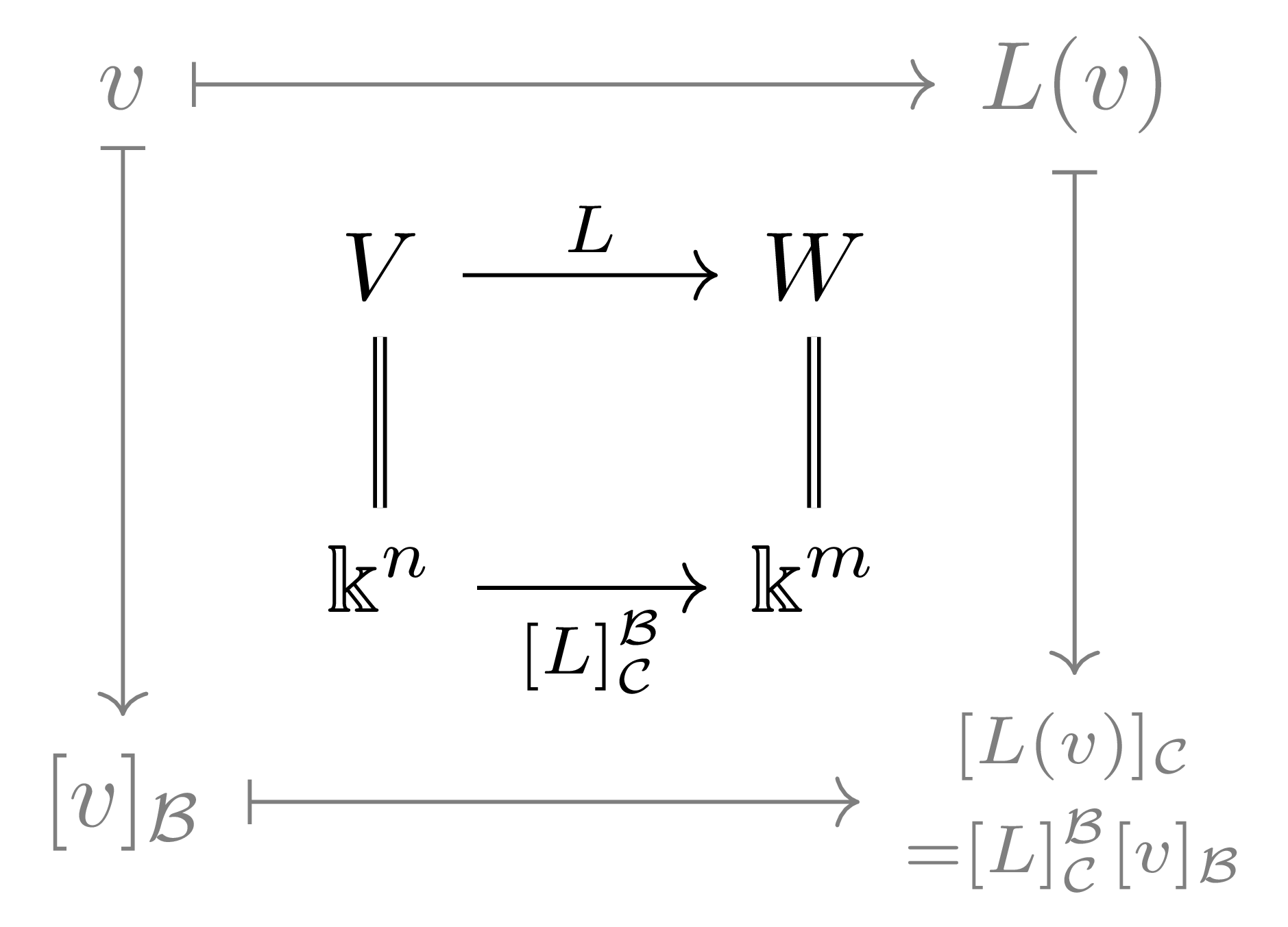
\[v=\sum_{i=1}^n v_ix_i\mapsto [v]_\mathcal{B}=\begin{pmatrix}v_1\\v_2\\\vdots\\v_n\end{pmatrix}\in\mathbb{K}^n\]Similarly, let another finite-dimensional $\mathbb{K}$-vector space $W$ and its basis $\mathcal{C}={y_1,\ldots, y_m}$ be given, and suppose the linear map $L:V\rightarrow W$ is determined by the following equations
\[\begin{aligned}L(x_1)&=\alpha_{1,1}y_1+\alpha_{2,1}y_2+\cdots+\alpha_{m,1}y_m\\L(x_2)&=\alpha_{1,2}y_1+\alpha_{2,2}y_2+\cdots+\alpha_{m,2}y_m\\&\vdots\\L(x_n)&=\alpha_{1,n}y_1+\alpha_{2,n}y_2+\cdots+\alpha_{m,n}y_m\end{aligned}\]Then we define the matrix representation $[L]^\mathcal{B}_\mathcal{C}$ of $L$ with respect to $\mathcal{B},\mathcal{C}$ this time by the following equation
\[[L]^\mathcal{B}_\mathcal{C}=\begin{pmatrix}\alpha_{1,1}&\alpha_{1,2}&\cdots&\alpha_{1,n}\\\alpha_{2,1}&\alpha_{2,2}&\cdots&\alpha_{2,n}\\\vdots&\vdots&\ddots&\vdots\\\alpha_{m,1}&\alpha_{m,2}&\cdots&\alpha_{m,n}\end{pmatrix}\]Comparing equations (2) and (1), one can check that for any $v\in V$, the coordinate representation of $L(v)$ with respect to $\mathcal{C}$ is given by the following equation
\[[L(v)]_\mathcal{C}=[L]^\mathcal{B}_\mathcal{C}[v]_\mathcal{B}\tag{3}\]Then the general version of Theorem 2 is given by the following theorem.
Theorem 4 \(\Hom(V,W)\cong \Mat_{m\times n}(\mathbb{K})\).
Proof
Fix bases $\mathcal{B}$ and $\mathcal{C}$ of $V$ and $W$ respectively. We need to show that the map $L\mapsto[L]^\mathcal{B}_\mathcal{C}$ is linear.
Let $L_1,L_2$ both be elements of $\Hom(V,W)$. Then for each $x_i\in\mathcal{B}$,
\[\begin{aligned}L_1(x_1)&=\alpha_{1,1}y_1+\alpha_{2,1}y_2+\cdots+\alpha_{m,1}y_m\\L_1(x_2)&=\alpha_{1,2}y_1+\alpha_{2,2}y_2+\cdots+\alpha_{m,2}y_m\\&\vdots\\L_1(x_n)&=\alpha_{1,n}y_1+\alpha_{2,n}y_2+\cdots+\alpha_{m,n}y_m\end{aligned}\]and
\[\begin{aligned}L_2(x_1)&=\beta_{1,1}y_1+\beta_{2,1}y_2+\cdots+\beta_{m,1}y_m\\L_2(x_2)&=\beta_{1,2}y_1+\beta_{2,2}y_2+\cdots+\beta_{m,2}y_m\\&\vdots\\L_2(x_n)&=\beta_{1,n}y_1+\beta_{2,n}y_2+\cdots+\beta_{m,n}y_m\end{aligned}\]there exist families of scalars $(\alpha_{i,j})$ and $(\beta_{i,j})$ such that these equations hold. Now,
\[\begin{aligned}(L_1+L_2)(x_1)&=(\alpha_{1,1}+\beta_{1,1})y_1+(\alpha_{2,1}+\beta_{2,1})y_2+\cdots+(\alpha_{m,1}+\beta_{m,1})y_m\\(L_1+L_2)(x_2)&=(\alpha_{1,2}+\beta_{1,2})y_1+(\alpha_{2,2}+\beta_{2,2})y_2+\cdots+(\alpha_{m,2}+\beta_{m,2})y_m\\&\vdots\\(L_1+L_2)(x_n)&=(\alpha_{1,n}+\beta_{1,n})y_1+(\alpha_{2,n}+\beta_{2,n})y_2+\cdots+(\alpha_{m,n}+\beta_{m,n})y_m\end{aligned}\]will hold, and thus the matrix representation $[L_1+L_2]^\mathcal{B}\mathcal{C}$ of $L_1+L_2$ is exactly $[L_1]^\mathcal{B}\mathcal{C}+[L_2]^\mathcal{B}_\mathcal{C}$. Similarly, the same holds for scalar multiplication.
Theorem 3 also has a similar generalization.
Theorem 5 Let three $\mathbb{K}$-vector spaces $V_1,V_2,V_3$ and their respective bases $\mathcal{B}_1={x_1,\ldots,x_n}$, $\mathcal{B}_2={y_1,\ldots, y_m}$, $\mathcal{B}_3={z_1,\ldots, z_k}$ be given. Then for any $L_1:V_1\rightarrow V_2$, $L_2:V_2\rightarrow V_3$ we always have
\[[L_2\circ L_1]^{\mathcal{B}_1}_{\mathcal{B}_3}=[L_2]^{\mathcal{B}_2}_{\mathcal{B}_3}[L_1]^{\mathcal{B}_1}_{\mathcal{B}_2}\]That is, the composition of linear maps equals the product of matrices.
Proof
To determine the left-hand side $[L_2\circ L_1]^{\mathcal{B}1}{\mathcal{B}_3}$, it suffices to check where the elements of $\mathcal{B}_1$ are mapped by $L_2\circ L_1$. Suppose $L_1$, $L_2$ are given by the following equations
\[[L_1]^{\mathcal{B}_1}_{\mathcal{B}_2}=\begin{pmatrix}\alpha_{1,1}&\alpha_{1,2}&\cdots&\alpha_{1,n}\\\alpha_{2,1}&\alpha_{2,2}&\cdots&\alpha_{2,n}\\\vdots&\vdots&\ddots&\vdots\\\alpha_{m,1}&\alpha_{m,2}&\cdots&\alpha_{m,n}\end{pmatrix},\quad[L_2]^{\mathcal{B}_2}_{\mathcal{B}_3}=\begin{pmatrix}\beta_{1,1}&\beta_{1,2}&\cdots&\beta_{1,m}\\\beta_{2,1}&\beta_{2,2}&\cdots&\beta_{2,m}\\\vdots&\vdots&\ddots&\vdots\\\beta_{k,1}&\beta_{k,2}&\cdots&\beta_{k,m}\end{pmatrix}\]A short calculation yields,
\[\begin{aligned}(L_2\circ L_1)(x_i)&=L_2(\alpha_{1,i}y_1+\cdots+\alpha_{m,i}y_m)\\&=\alpha_{1,i}L_2(y_1)+\alpha_{2,i}L_2(y_2)+\cdots+\alpha_{m,i}L(y_m)\\&=\alpha_{1,i}(\beta_{1,1}z_1+\beta_{2,1}z_2+\cdots+\beta_{k,1}z_k)\\&\phantom{==}+\alpha_{2,i}(\beta_{1,2}z_1+\beta_{2,2}z_2+\cdots+\beta_{k,2}z_k)\\&\phantom{===}+\cdots\\&\phantom{====}+\alpha_{m,i}(\beta_{1,m}z_1+\beta_{2,m}z_2+\cdots+\beta_{k,m}z_k)\end{aligned}\]Now, grouping the above expression by the $z$’s, we obtain
\[(L_2\circ L_1)(x_i)=\left(\sum_{l=1}^m\alpha_{l,i}\beta_{1,l}\right)z_1+\cdots+\left(\sum_{l=1}^m\alpha_{l,i}\beta_{k,l}\right)z_k\]Since we already checked that the $i$-th column of $[L_2\circ L_1]^{\mathcal{B}1}{\mathcal{B}3}$ is exactly the coordinate representation in $\mathcal{B}_3$ of the vector to which $x_i$ is mapped by $L_2\circ L_1$, the entry in row $j$, column $i$ of the matrix $[L_2\circ L_1]^{\mathcal{B}_1}{\mathcal{B}3}$ is the $j$-th component $\sum{l=1}^m\alpha_{l,i}\beta_{j,l}$ of this vector. Just as in Theorem 3, this component is the $(i,j)$ entry of the matrix product $[L_2]^{\mathcal{B}2}{\mathcal{B}3}[L_1]^{\mathcal{B}_1}{\mathcal{B}_2}$, so the proof is complete.
Theorem 4 above shows that once we choose bases for $V,W$, we can regard $\Hom(V,W)$ and $\Mat_{m\times n}(\mathbb{K})$ as the same. For example, the $mn$ basis elements of $\Mat_{m\times n}(\mathbb{K})$ correspond to the $mn$ basis elements we examined in §The Space of Linear Maps, ⁋Proposition 5. The following corollary is also a consequence of the fundamental theorem.
Corollary 6 Let two $n$-dimensional $\mathbb{K}$-vector spaces $V,W$ be given, and fix their bases $\mathcal{B},\mathcal{C}$. Then for any $L\in\Hom(V,W)$, the matrix representation $[L^{-1}]^{\mathcal{C}}{\mathcal{B}}$ of $L^{-1}\in\Hom(W,V)$ with respect to the bases $\mathcal{C},\mathcal{B}$ equals the inverse matrix of $[L]^{\mathcal{B}}\mathcal{C}$.
Proof
Obvious from the uniqueness of inverse matrices and inverse functions.
In this way, most concepts defined in §Matrices can be transferred to $\Hom(V,W)$. One concept that cannot be transferred immediately is the transpose matrix $A^t$; we will understand its meaning later when we examine dual spaces.
Change-of-Basis Matrices
To sum up Theorem 4 in one sentence: a linear map from an $n$-dimensional vector space $V$ to an $m$-dimensional vector space $W$ can be represented by an $m\times n$ matrix once bases $\mathcal{B},\mathcal{C}$ of them are fixed, and conversely any $m\times n$ matrix can be understood as a linear map.
Then one natural question is what happens when we change the basis, and in fact the answer is already given in Theorem 5.
Definition 7 For an arbitrary finite-dimensional $\mathbb{K}$-vector space $V$ and two bases $\mathcal{B},\mathcal{B}’$ of $V$, the change-of-basis matrix from $\mathcal{B}$ to $\mathcal{B}’$ means
\[[\id_V]_{\mathcal{B}'}^\mathcal{B}\]It is obvious from the fact that the dimension of a vector space is well defined that such a matrix must be a square matrix. Also, from the following equation
\[I=[\id_V]^{\mathcal{B}}_{\mathcal{B}}=[\id_V]_{\mathcal{B}}^{\mathcal{B}'}[\id_V]^\mathcal{B}_{\mathcal{B}'}\]we see that such a matrix is always invertible.
To see how a change-of-basis matrix works, fix a finite-dimensional $\mathbb{K}$-vector space $V$ and let two bases $\mathcal{B},\mathcal{B}’$ of $V$ be given. The fundamental theorem of linear algebra means that the following diagram commutes.
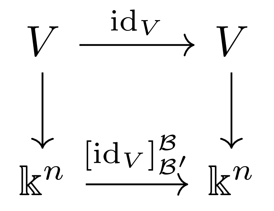
Here the two vertical maps mean $v\mapsto [v]\mathcal{B}$ and $v\mapsto[v]{\mathcal{B}’}$ respectively. Therefore, one can think of the change-of-basis matrix as a matrix that takes the coordinate representation of $v\in V$ with respect to $\mathcal{B}$ and converts it to the coordinate representation with respect to $\mathcal{B}’$.
More generally, let an arbitrary linear map $L:V\rightarrow W$ be given, and let bases $\mathcal{B},\mathcal{C}$ of $V,W$ and other bases $\mathcal{B}’,\mathcal{C}’$ be given. Then from the fundamental theorem of linear algebra we obtain the following equation
\[[L]_{\mathcal{C}'}^{\mathcal{B}'}=[\id_W]_{\mathcal{C}'}^\mathcal{C}[L]_{\mathcal{C}}^\mathcal{B}[\id_V]^{\mathcal{B}'}_{\mathcal{B}}\]Let two $m\times n$ matrices $A,B$ be given. Then from the above equation, if there exist suitable invertible matrices $P,Q$ satisfying the following equation
\[B=PAQ\]one feels tempted to regard $A$ and $B$ as the same. This means regarding all matrix representations obtained by choosing bases of the domain and codomain of a fixed linear map $L$ as the same.
However, despite this plausible motivation, the outcome is rather poor. If one can change both the domain and codomain bases of $L$, one can choose an arbitrary basis ${x_1,\ldots, x_n}$ of the domain, then select the linearly independent elements $L(x_1),\ldots, L(x_k)$ from among $L(x_1),\ldots, L(x_n)$ and use §Dimension of Vector Spaces, ⁋Proposition 6 to make a basis of the codomain, because then this linear map can always be represented in the block matrix form
\[\begin{pmatrix}I&O\\O&O\end{pmatrix}\]That is, if we classify matrix representations of $L$ in this way, the only thing that affects the classification is the rank of $L$.
Therefore, we need to define a finer relation than this equivalence relation.
Definition 8 Let arbitrary $n\times n$ matrices $A,B$ be given. Then $A$ and $B$ are called similar matrices if there exists a suitable invertible matrix $P$ such that $A=PBP^{-1}$ holds.
In other words, saying that matrices $A,B$ are similar means that when we think of $A$ as the matrix representation of the linear transformation $L:V\rightarrow V$ with respect to a basis $\mathcal{B}$, there exists a suitable basis $\mathcal{C}$ such that $B$ can be thought of as the matrix representation of $L$ with respect to basis $\mathcal{C}$. Then at this time
\[A=[L]_{\mathcal{B}}^\mathcal{B}=[\id_V]^\mathcal{B}_\mathcal{C}[L]^\mathcal{C}_\mathcal{C}[\id_V]^\mathcal{C}_\mathcal{B}=PBP^{-1}\]holds.
References
[Lee] 이인석, 선형대수와 군, 서울대학교 출판문화원, 2005.
-
Unlike the fundamental theorem of calculus, the fundamental theorem of algebra, etc., the fundamental theorem of linear algebra can mean completely different theorems depending on the author. For example, in [Goc] the rank-nullity theorem from the previous post is called the fundamental theorem of linear algebra, and in Gilbert Strang’s case the theorems on orthogonal complements that we will cover in the next post are so called. We follow [Lee] in calling this theorem the fundamental theorem of linear algebra. ↩
댓글남기기