
This post was machine-translated from Korean by Kimi CLI. The translation may contain errors. The Korean original is the source of truth.
As in differential geometry, the tangent space is a central tool in algebraic geometry for understanding the local structure of varieties.
Definition of the Tangent Space
In differential geometry, for the sheaf \(\mathcal{C}^\infty_M\) of smooth functions defined on \(M\), we verified that the collection of all germs vanishing at a point \(x\in M\),
\[\mathfrak{m}_x=\{\mathbf{f}\in \mathcal{C}^\infty_x\mid \mathbf{f}(x)=0\}\]is a maximal ideal. We then proved that the tangent space can be viewed as
\[(\mathfrak{m}_x/\mathfrak{m}_x^2)^\ast\]([Differentiable Manifolds] §Cotangent Spaces, ⁋Lemma 1). This construction is not usually emphasized in differential geometry, but it is extremely helpful for generalizing to algebraic varieties. Namely, (fixing the affine case for convenience) we already know what functions defined on algebraic varieties are (§Quasi-Projective Varieties, ⁋Definition 7), and we also know that the collection of all functions vanishing at \(x\in X\) corresponds to the maximal ideal of \(\mathbb{K}[X]\) at this point. Therefore we define
\[\mathfrak{m}_x=\{f\in \mathbb{K}[X]\mid f(x)=0\}\]and can consider the localization \(\mathbb{K}[X]_{\mathfrak{m}_x}=\mathcal{O}_{X,x}\) of \(\mathbb{K}[X]\) at this maximal ideal ([Commutative Algebra] §Localization, ⁋Definition 1). Geometrically, by §Affine Varieties, ⁋Definition 14, these can be defined as germs of regular functions at the point \(x\).
Definition 1 We define the Zariski tangent space \(T_x X\) of a variety \(X\) at a point \(x\) by
\[T_x X = (\mathfrak{m}_x / \mathfrak{m}_x^2)^\ast\]where \(\mathfrak{m}_x\) is the unique maximal ideal of the local ring \(\mathcal{O}_{X,x}\) at the point \(x\).
The essence of this definition is that the quotient \(\mathfrak{m}_x / \mathfrak{m}_x^2\) carries the first-order infinitesimal data at \(x\), so we define it to be the Zariski cotangent space \(T_x^\ast X\). The dual \(T_x X\) is the space of linear functionals acting on this data—that is, directional derivative operators—and this definition coincides with defining \(T_xX=\Der_\mathbb{K}(\mathcal{O}_{X,x}, \mathbb{K})\).
We do not use the analysis-style \(\epsilon\)-\(\delta\) differential, but essentially varieties are defined by polynomials, and their differentiation can be thought of formally as differentiating \(\x^n\) to obtain \(n\cdot \x^{n-1}\). In particular, for an affine variety this can be written more explicitly.
Proposition 2 For an affine variety \(X = Z(f_1, \ldots, f_k) \subseteq \mathbb{A}^n\) and a point \(x = (x_1, \ldots, x_n)\),
\[T_x X \cong \{v \in \mathbb{K}^n \mid (df_i)_x(v) = 0 \text{ for all } i\}\]Here \((df_i)_x\) is the differential of \(f_i\) at \(x\),
\[(df_i)_x(v) = \sum_{j=1}^n \frac{\partial f_i}{\partial \x_j}(x) v_j\]Proof
Consider the coordinate ring \(\mathbb{K}[X] = \mathbb{K}[\x_1, \ldots, \x_n] / (f_1, \ldots, f_k)\) of \(X\). Since \(\mathfrak{m}_x = (\x_1 - a_1, \x_2 - a_2, \ldots, \x_n - a_n) / (f_1, \ldots, f_k)\),
\[\mathfrak{m}_x / \mathfrak{m}_x^2 \cong (\x_1 - a_1, \x_2 - a_2, \ldots, \x_n - a_n) / \left( (\x_1 - a_1, \x_2 - a_2, \ldots, \x_n - a_n)^2 + (f_1, \ldots, f_k) \right)\]Expanding each \(f_i\) in a Taylor series at \(x\) gives
\[f_i = \sum_{j=1}^n \frac{\partial f_i}{\partial \x_j}(x) (\x_j - a_j) + \text{higher order terms}\]and the higher order terms lie in \((\x_1 - a_1, \x_2 - a_2, \ldots, \x_n - a_n)^2\). Hence in \(\mathfrak{m}_x / \mathfrak{m}_x^2\) the linear parts \(\sum_j \frac{\partial f_i}{\partial \x_j}(x) (\x_j - a_j)\) of the \(f_i\) vanish.
On the other hand, \(\mathfrak{m}_x / \mathfrak{m}_x^2\) is generated by linear combinations of the \(\x_j - a_j\), so it can be viewed as a quotient of \(\mathbb{K}^n\). The kernel of the differential \((df_i)_x\) then corresponds exactly to the directions that disappear in \(\mathfrak{m}_x / \mathfrak{m}_x^2\). Taking the dual yields
\[T_x X = (\mathfrak{m}_x / \mathfrak{m}_x^2)^\ast \cong \{v \in \mathbb{K}^n \mid (df_i)_x(v) = 0 \text{ for all } i\}\]Although the proof is written in the language of maximal ideals and looks complicated, its philosophy is simple when one thinks of \(X=Z(f_i)\). In this case \((df_i)_x(v)=0\) is precisely the (ordinary) tangent space of the hypersurface \(Z(f_i)\) in \(\mathbb{A}^n\) (viewing \(\mathbb{K}^n\) as \(\mathbb{A}^n\)). Proposition 2 applies only to affine varieties as stated, but any point \(x\) of an arbitrary variety \(X\) has an affine neighborhood, so it essentially applies to all varieties. The same is true of the next proposition concerning the dimension of the tangent space.
Proposition 3 \(T_x X\) is a \(\mathbb{K}\)-vector space, and its dimension is \(n - \operatorname{rank}(J_x)\). Here \(J_x\) is the \(k \times n\) Jacobian matrix
\[J_x = \left(\frac{\partial f_i}{\partial \x_j}(x)\right)_{1 \le i \le k, 1 \le j \le n}\]Proof
Each \((df_i)_x: \mathbb{K}^n \to \mathbb{K}\) is a linear functional. By Proposition 2, \(T_x X\) is the intersection of their kernels, hence a subspace of \(\mathbb{K}^n\). The rows of the Jacobian matrix \(J_x\) are the coordinate representations of these linear functionals, so
\[T_x X = \ker(J_x) = \{v \in \mathbb{K}^n \mid J_x v = 0\}\]By the rank-nullity theorem, \(\dim T_x X = n - \operatorname{rank}(J_x)\).
Smooth and Singular Points
In differential geometry, the dimension of the tangent space at any point was always equal to the dimension of the manifold. Yet this is because the definition of a manifold is rather stringent; in algebraic geometry, even an affine variety defined by a single polynomial may fail to be a manifold (in the classical sense). (Example 6, Example 7) Nonetheless, the dimension of the tangent space is not unrelated to the dimension of the variety.
Proposition 4 For any point \(x\) of an irreducible variety \(X\), \(\dim T_x X \ge \dim X\).
Proof
We prove only the affine case. Let \(X = Z(f_1, \ldots, f_k) \subseteq \mathbb{A}^n\) be irreducible with \(\dim X = d\). Consider the local ring \(\mathcal{O}_{X,x} = \mathbb{K}[X]_{\mathfrak{m}_x}\) at the point \(x \in X\). Localization preserves dimension, so \(\dim \mathcal{O}_{X,x} = \dim X = d\). ([Algebraic Varieties] §Dimension, ⁋Proposition 2)
In general, for a Noetherian local ring \((R, \mathfrak{m})\) one has \(\dim_{\mathbb{K}}(\mathfrak{m}/\mathfrak{m}^2) \ge \dim R\). ([Commutative Algebra] §Systems of Parameters, ⁋Proposition 2) Therefore
\[\dim T_x X = \dim_{\mathbb{K}}(\mathfrak{m}_x/\mathfrak{m}_x^2) \ge \dim \mathcal{O}_{X,x} = d = \dim X\]To sharpen our intuition, it is helpful to look at when the inequality is strict. We call such points singular points.
Definition 5 A point \(x \in X\) is a smooth point (or nonsingular point) if \(\dim T_x X = \dim X\). Otherwise (that is, if \(\dim T_x X > \dim X\)) it is called a singular point.
Example 6 (Smooth points)
- Every point of \(\mathbb{A}^n\) is a smooth point. Since \(\mathbb{A}^n\) has no defining equations, \(T_x \mathbb{A}^n = \mathbb{K}^n\), and \(\dim T_x \mathbb{A}^n = n = \dim \mathbb{A}^n\).
- Every point of the parabola \(Z(\y - \x^2)\) is a smooth point. For \(f = \y - \x^2\) we have \(J_{(x,y)} = (-2x, 1)\), which is nonzero at every point. Hence \(\dim T_x X = 2 - 1 = 1 = \dim X\).
Example 7 (Singular points)
-
(Node) Let \(X = Z(\y^2 - \x^2(\x+1)) \subset \mathbb{A}^2\). This curve splits into two branches at the origin.
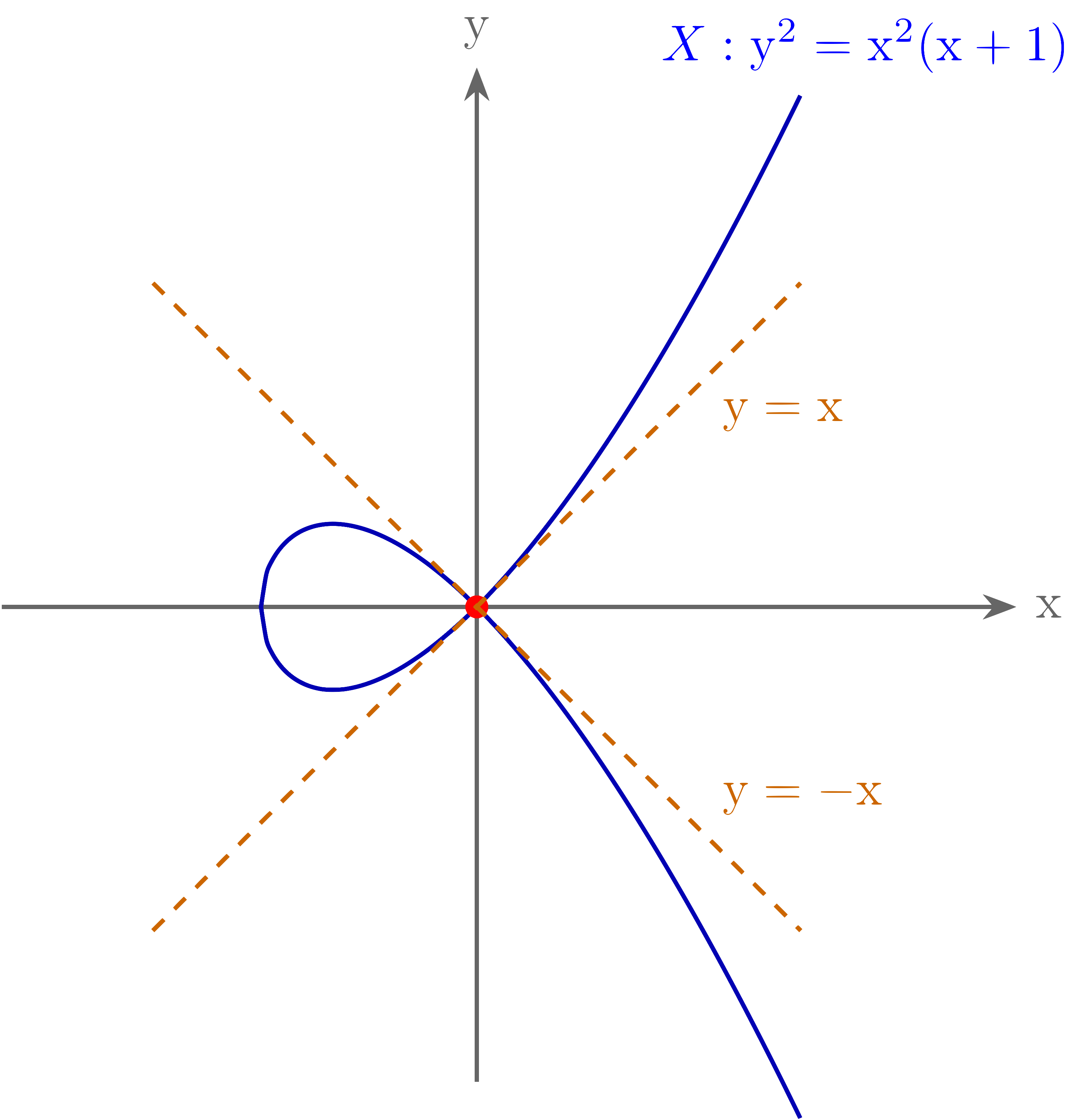
The Jacobian of this curve is
\[J_{(x,y)} = \begin{pmatrix} -2x - 3x^2 & 2y \end{pmatrix}\]so at the origin the Jacobian is \((0,0)\), and therefore the origin is a singular point by Proposition 3. Geometrically, the tangent space being two-dimensional means that both tangent directions of the two branches are included. Concretely, since \(\y^2 - \x^2(\x+1) \approx \y^2 - \x^2 = (\y-\x)(\y+\x)\), near the origin the curve looks like the union of the two lines \(\y = \x\) and \(\y = -\x\). A node is one of the “mildest” singularities.
-
(Cusp) Now consider \(Z(\y^2 - \x^3)\subset \mathbb{A}^2\).
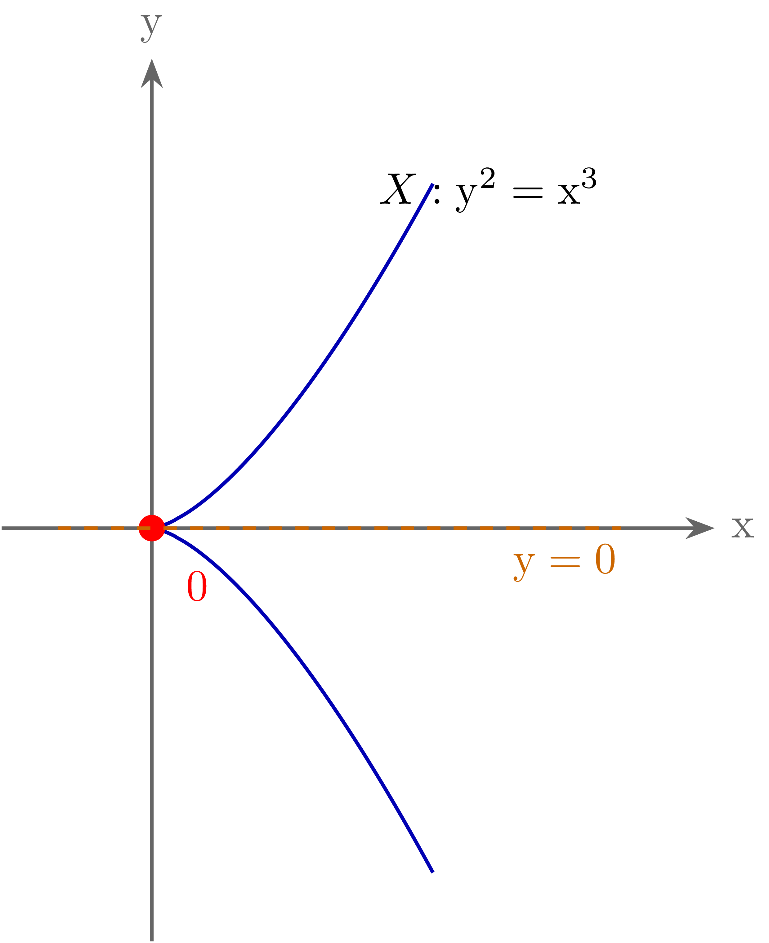
In this case the origin of this curve is a singular point. Computing the Jacobian,
\[J_{(x,y)}=\begin{pmatrix}-3x^2&2y\end{pmatrix}\]so \(\nabla f(0,0) = (0, 0)\) at the origin. Geometrically, the fact that the tangent space is two-dimensional here means that every direction is “tangent” at the origin, indicating that the curve is too sharp for a tangent line to be defined in any direction.
In the examples above we naturally used the following proposition.
Proposition 8 (Jacobian Criterion) Let \(X = Z(f_1, \ldots, f_k) \subseteq \mathbb{A}^n\) be irreducible and let \(x \in X\). Then \(x\) is a smooth point if and only if the Jacobian matrix \(J_x\) has rank \(n - \dim X\).
Proof
Proposition 2 showed that \(\dim T_x X = n - \operatorname{rank}(J_x)\). By Definition 5, \(x\) is a smooth point if and only if \(\dim T_x X = \dim X\). Therefore \(x\) is a smooth point if and only if
\[n - \operatorname{rank}(J_x) = \dim X\]that is, \(\operatorname{rank}(J_x) = n - \dim X\).
Existence of Smooth Points
Any algebraic variety is smooth at most points. To show this we need the notion of a generic point.
Definition 9 The generic point \(\eta\) of an irreducible variety \(X\) is the unique point belonging to every nonempty open subset of \(X\).
In the affine case \(X = \operatorname{Spec} A\), \(\eta\) corresponds to the minimal prime ideal of \(A\) (namely, the \((0)\) ideal), and the local ring \(\mathcal{O}_{X,\eta}\) is precisely the function field \(\mathbb{K}(X) = \operatorname{Frac}(A)\). Geometrically, the generic point is the “most general” point of \(X\), a point that has no particular property of \(X\). We can use this idea in the following proof.
Proposition 10 The set \(X_\sm\) of smooth points of a variety \(X\) is a dense open subset of \(X\). In particular, \(X_\sm \ne \emptyset\).
Proof
Let \(X = Z(f_1, \ldots, f_k) \subseteq \mathbb{A}^n\) have dimension \(\dim X = d\). By the Jacobian criterion of Proposition 8,
\[X_\sm = \{x \in X \mid \operatorname{rank}(J_x) = n - d\}\]We show that this set is a dense open subset. First, it is relatively obvious that \(X_\sm\) is open. Having rank exactly \(n-d\) means that two conditions hold simultaneously. First, having rank at least \(n-d\) is equivalent to some \((n-d) \times (n-d)\) minor being nonzero, which is an open condition in the Zariski topology. Second, having rank at most \(n-d\) is equivalent to every \((n-d+1) \times (n-d+1)\) minor vanishing, which is a closed condition. Hence the set of points where the rank is exactly \(n-d\) is an open subset of \(X\).
Showing that \(X_\sm\) is nonempty is somewhat technical. The idea is that a generic point should be smooth, so we consider the generic point \(\eta\) of \(X\). Thinking of the localization at \(\eta\), the local ring \(\mathcal{O}_{X,\eta} = \mathbb{K}(X)\) is a field, hence a regular local ring. By [Commutative Algebra] §Systems of Parameters, ⁋Proposition 2,
\[\dim_{\mathbb{K}}(\mathfrak{m}_\eta/\mathfrak{m}_\eta^2) \ge \dim \mathcal{O}_{X,\eta} = d\]while the reverse inequality also holds by Proposition 4, so \(\dim T_\eta X = d\). Therefore \(\eta \in X_\sm\). Now any nonempty open subset is dense by irreducibility.
We now give the following definition.
Definition 11 A variety \(X\) is smooth (or nonsingular) if every point is a smooth point, i.e., \(X_\sm = X\). Otherwise (that is, if a singular point exists) it is called singular.
Example 12 The varieties in Example 6 are all smooth, and all the varieties in Example 7 are singular.
Tangent Cones
At a singular point the tangent space is too large to reflect the local structure of the variety accurately. In this case the tangent cone provides more accurate information. Intuitively, the tangent space is too large because the Jacobian has too small a rank; this happens, for example, when the first-order approximation of the given function carries no information. Thus, if we consider higher-order approximations of the given function, the situation may change.
To this end, for any polynomial \(f\in \mathbb{K}[\x_1,\ldots, \x_n]\) we define the initial term \(\initial(f)\) of \(f\) to be the homogeneous component of \(f\) of least degree. Then for any ideal \(\mathfrak{a}\), the initial ideal \(\initial(\mathfrak{a})\) is defined to be the homogeneous ideal generated by the \(\initial(f)\).
Definition 13 For any affine variety \(X\subseteq \mathbb{A}^n\), the algebraic variety defined by \(\initial(I(X))\) is called the tangent cone of \(X\) at the origin.
More generally, by writing \(f\) as a polynomial in the \(\x_i-x_i\) and making the analogous definition, one can define the tangent cone at an arbitrary point. It is called a cone because, as in §Projective Varieties, ⁋Definition 12, it is the zero set of a homogeneous ideal.
Now let us see how this classifies singular points more finely.
Example 14 For the nodal curve \(X = Z(\y^2 - \x^2(\x+1))\) of Example 7, the lowest-degree term of \(f\) is \(\y^2 - \x^2 = (\y-\x)(\y+\x)\), so
\[TC_0 X = Z(\y-\x) \cup Z(\y+\x)\]This exactly shows that the node splits in the directions of the two lines \(\y = \x\) and \(\y = -\x\).
Example 15 For the curve \(X = Z(\y^2 - \x^3)\) of Example 7, the lowest-degree term of \(f\) is \(\y^2\), so
\[TC_0 X = Z(\y^2)\]This is the line \(\y = 0\) counted twice, showing that the cusp ends sharply along the \(\x\)-axis. By comparison, the tangent space \(T_0 X = \mathbb{K}^2\) contains every direction and is too large.
In general, as we saw in §Rational Maps, ⁋Example 12, the singularity of a nodal curve can be resolved by a blowup: after blowing up, the two lines \(\y-\x\) and \(\y+\x\) at the origin are separated by \(\mathbb{P}^1\). However, a cusp cannot be resolved in this way, so in general a cusp is regarded as a worse singularity than a node.
References
[Har] J. Harris, Algebraic Geometry: A First Course, Springer, 1992. [Sha] I. R. Shafarevich, Basic Algebraic Geometry I: Varieties in Projective Space, Springer, 2013.
댓글남기기