
This post was machine-translated from Korean by Kimi CLI. The translation may contain errors. The Korean original is the source of truth.
Previously, we defined a (Weil) divisor on a variety \(X\) in §Divisors, ⁋Definition 1. By the definition of the Zariski topology, this can basically be thought of as the zero set of some function defined on \(X\), with the orders of these zeros added in, and to make this well defined even in cases such as \(\mathbb{P}^n\) we generalized functions to sections of a suitable line bundle.
On the other hand, since divisors also allow negative coefficients, this zero set may not be a zero set but rather a zero of negative order, that is, a pole. In this case, we can find an effective divisor linearly equivalent to the given divisor and then study this property. (§Divisors, ⁋Definition 7)
Above, for convenience of exposition, we discussed only Weil divisors, but a similar argument works for Cartier divisors, and the resulting definition is as follows.
Definition 1 A Weil divisor \(D=\sum n_i D_i\) defined on a variety \(X\) is effective if \(n_i \geq 0\) for all \(i\). A Cartier divisor \(\{(U_i, f_i)\}\) is effective if \(f_i\) is regular on \(U_i\) for all \(i\).
Then our goal is to examine whether any effective divisors exist in the divisor class of \(D\). To this end, consider the line bundle \(\mathcal{L}=\mathcal{O}_X(D)\) defined by the divisor \(D\). (§Line Bundles and Vector Bundles, ⁋Definition 17) Each nonzero global section \(s\in \Gamma(X, \mathcal{L})\) of \(\mathcal{L}\) has no poles, so it defines an effective divisor \(\divisor(s)\), and we can check that this differs from the original \(D\) only by a trivialization, so it is linearly equivalent to \(D\). Thus, to find an effective divisor linearly equivalent to \(D\), it suffices to look at nonzero global sections of \(\mathcal{O}_X(D)\). However, the point to note is that \(\divisor(s)\) depends not on \(s\) itself but on its nonzero scalar multiples, and therefore the object we should be interested in is not \(\Gamma(X, \mathcal{L})\) itself but its projectivization.
Definition 2 For a line bundle \(\mathcal{L}\) on a variety \(X\), the complete linear system of \(\mathcal{L}\) is the projectivization of the global section space \(\Gamma(X, \mathcal{L})\) of \(\mathcal{L}\):
\[\lvert \mathcal{L} \rvert = \mathbb{P}(\Gamma(X, \mathcal{L})).\]A linear system for \(\mathcal{L}\) is a nonempty projective subspace of \(\lvert \mathcal{L} \rvert\). That is, it is of the form \(\mathbb{P}(V) \subseteq \lvert \mathcal{L} \rvert\) for a subspace \(V \subseteq \Gamma(X, \mathcal{L})\).
Linear System on Projective Space
By the calculations following §Line Bundles and Vector Bundles, ⁋Example 12, we saw that \(\Gamma(\mathbb{P}^n, \mathcal{O}_{\mathbb{P}^n}(d))\) is isomorphic to the space of homogeneous polynomials of degree \(d\), \(\mathbb{K}[\x_0, \ldots, \x_n]_d\). Since each element of this space defines a degree \(d\) hypersurface in \(\mathbb{P}^n\), we can understand the complete linear system
\[\lvert \mathcal{O}_{\mathbb{P}^n}(d)\rvert=\mathbb{P}(\Gamma(\mathbb{P}^n, \mathcal{O}_{\mathbb{P}^n}(d)))\cong \mathbb{P}(\mathbb{K}[\x_0,\ldots, \x_n]_d)\cong \mathbb{P}^{\binom{n+d}{d} - 1}\]geometrically as a family of degree \(d\) hypersurfaces in \(\mathbb{P}^n\).
Example 3 For convenience, fix \(n=2\). Then the family of degree \(1\) hypersurfaces, i.e., lines in \(\mathbb{P}^2\), is isomorphic to \(\mathbb{P}^2\) itself. Looking more closely,
\[\lvert \mathcal{O}_{\mathbb{P}^2}(1)\rvert\cong \mathbb{P}(\mathbb{K}[\x_0,\x_1,\x_2]_1)\cong \mathbb{P}^{\binom{3}{1}-1}=\mathbb{P}^2\]a point \([a_0:a_1:a_2]\) on the right-hand side \(\mathbb{P}^2\) defines a line \(Z(a_0\x_0+a_1\x_1+a_2\x_2)\) in \(\mathbb{P}^2\).
For a slightly more complicated and geometric example, consider a one-dimensional subspace (i.e., a one-dimensional linear system) of the complete linear system
\[\lvert \mathcal{O}_{\mathbb{P}^2}(2)\rvert\cong \mathbb{P}(\mathbb{K}[\x_0,\x_1,\x_2]_2)\cong \mathbb{P}^{\binom{3}{2}-1}=\mathbb{P}^5\]defined by the line bundle \(\mathcal{O}_{\mathbb{P}^2}(2)\) on \(\mathbb{P}^2\). A typical example is a pencil of two conics. Consider two conics \(C_1=Z(F_1)\), \(C_2=Z(F_2)\) defined in \(\mathbb{P}^2\). Then, unless \(C_1\) and \(C_2\) are the same conic, their linear combination
\[Z(\lambda F_1+\mu F_2)\]is another degree \(2\) curve in \(\mathbb{P}^2\), and by definition all these conics pass through \(C_1\cap C_2\). Here, the point \([\lambda:\mu]\in \mathbb{P}^1\) parametrizes these conics.
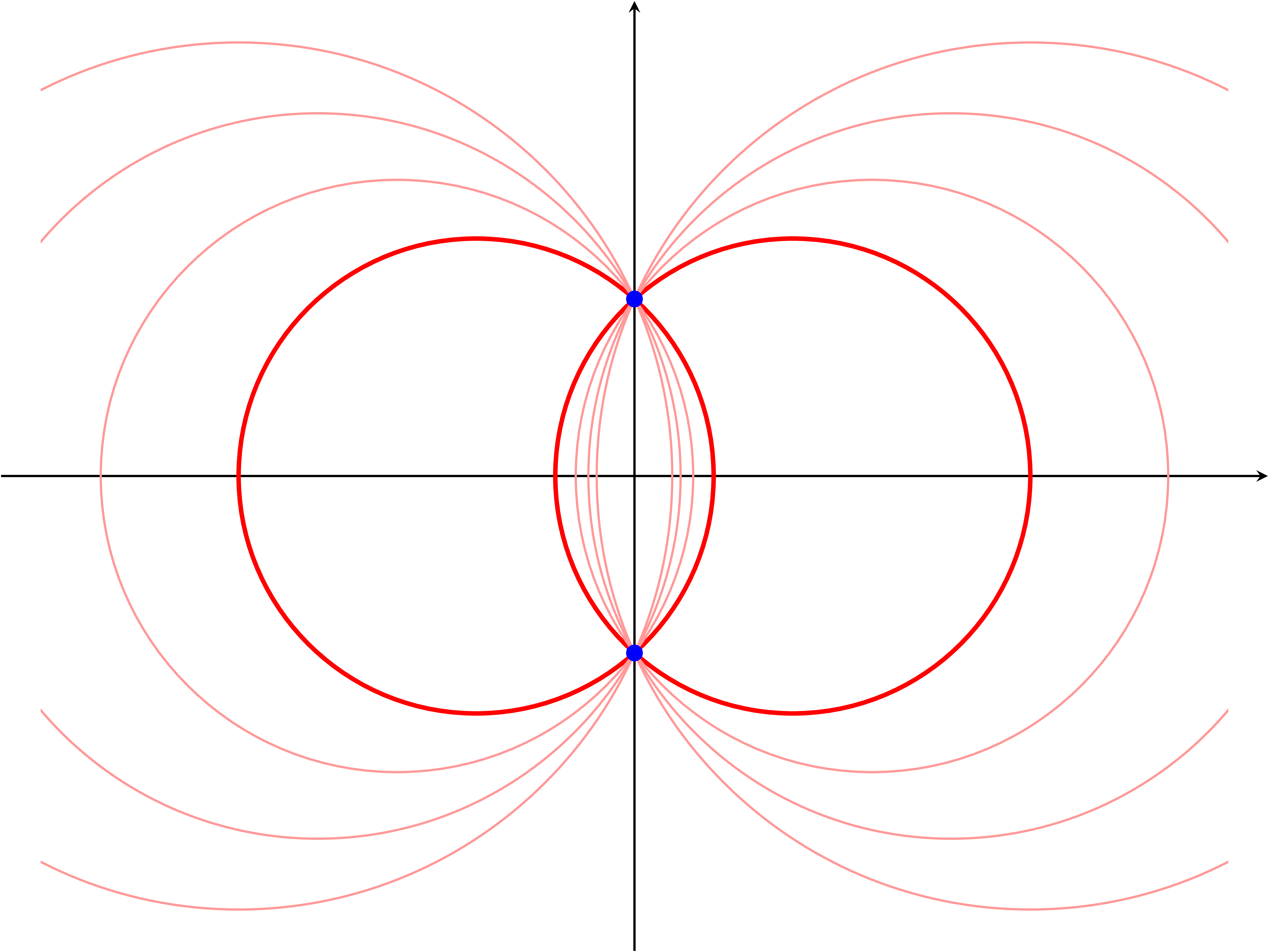
For a more concrete example, consider the two conics
\[C_1: Z((\x_0-2\x_2)^2+\x_1^2-9\x_2^2),\qquad C_2: Z((\x_0+2\x_2)^2+\x_1^2-9\x_2^2)\]in \(\mathbb{P}^2\). These equations look complicated as they are, but when restricted to \(U_2\) they become the equations of two circles
\[(\x-2)^2+\y^2=9,\qquad (\x+2)^2+\y^2=9.\]They meet at \((x,y)=(0,\pm\sqrt{5})\) on \(U_2\), which is computed from the two equations above, and outside \(U_2\) — that is, on the line at infinity of \(U_2\)1 — they meet at the two points \([1:i:0]\), \([1:-i:0]\). Then the above pencil \(Z(\lambda F_1+\mu F_2)\) is the collection of conics passing through their intersection \(C_1\cap C_2\).
Meanwhile, a general degree \(2\) homogeneous polynomial is of the form
\[F(\x_0,\x_1,\x_2) = a_{00}\x_0^2 + a_{11}\x_1^2 + a_{22}\x_2^2 + a_{01}\x_0\x_1 + a_{02}\x_0\x_2 + a_{12}\x_1\x_2,\]and this is exactly why \(\Gamma(X, \mathcal{O}(2))\) is a \(6\)-dimensional space. On the other hand, if we add the condition that it must pass through the four-point set \(C_1\cap C_2\) computed above, these four points each impose one constraint, eliminating one necessary parameter each, so we know there are \(2\) parameters representing this. More specifically, the following four conditions
\(0=F(0,\sqrt{5},1)=5a_{11}+a_{22}+\sqrt{5}a_{12}\) \(0=F(0,-\sqrt{5},1)=5a_{11}+a_{22}-\sqrt{5}a_{12}\) \(0=F(1,i,0)=a_{00}-a_{11}+ia_{01}\) \(0=F(1,-i,0)=a_{00}-a_{11}-ia_{01}\)
force \(a_{12}=0\), \(a_{01}=0\), \(5a_{11}=-a_{22}\), and \(a_{00}=a_{11}\), so the actual variables are the two \(a_{00}\) and \(a_{02}\). That is, this family of conics forms a \(2\)-dimensional subspace \(V\) of \(\Gamma(X,\mathcal{O}(2))\), and its projectivization becomes the \(\mathbb{P}^1\) represented by \([\lambda:\mu]\).
Of course, Definition 2 applies equally to any variety, whether \(X\) is projective space or a quasi-projective variety. However, the reason we took such pains with Example 3 above is that for any quasi-projective variety \(X\subseteq \mathbb{P}^n\), if \(D\) comes from some \(\mathcal{O}_{\mathbb{P}^n}(d)\), we can use the language of homogeneous polynomials as is. That is, in this case the restriction map
\[\Gamma(\mathbb{P}^n, \mathcal{O}_{\mathbb{P}^n}(d)) \to \Gamma(X, \mathcal{O}_{\mathbb{P}^n}(d)\vert_X)\]sends a homogeneous polynomial \(F \in \mathbb{K}[\x_0, \ldots, \x_n]_d\) to a section on \(X\), and its kernel is the degree \(d\) homogeneous part \(I(X)_d\) of \(I(X)\). Thus
\[\Gamma(X, \mathcal{O}_{\mathbb{P}^n}(d)\vert_X) \cong \mathbb{K}[\x_0, \ldots, \x_n]_d / I(X)_d\]so essentially the same calculations as in \(\mathbb{P}^n\) are possible. In particular, since \(F - G \in I(X)\) defines the same intersection, the parameter space becomes \(\mathbb{P}(V/(V \cap I(X)))\).
Base Locus
In the remainder of the post, given a linear system \(L=\mathbb{P}(V)\) on \(X\) and a basis \(F_0,\ldots,F_r\) of \(V\), we define the embedding
\[\varphi_L:X\rightarrow \mathbb{P}^r;\qquad x\mapsto [F_0(x):\cdots:F_r(x)]\]using it.
Of course, this is not always possible. For example, in Example 3, if we choose the following two basis elements
\[F_1(\x_0,\x_1,\x_2)=\x_0^2+\x_1^2-5\x_2^2, \qquad F_2(\x_0,\x_1,\x_2)=\x_0\x_2\]corresponding to \((a_{00},a_{02})=(1,0),(0,1)\), this “embedding” becomes
\[\mathbb{P}^2\rightarrow \mathbb{P}^1;\qquad [\x_0,\x_1,\x_2]\mapsto [\x_0^2+\x_1^2-5\x_2^2:\x_0\x_2].\]First, since this is a map from \(\mathbb{P}^2\) to the smaller space \(\mathbb{P}^1\), we know something is wrong, and this is because there is a locus where the two functions \(F_1,F_2\) vanish simultaneously.
The above embedding \(\varphi_L\) actually depends on the choice of basis of \(V\), but various properties that \(\varphi_L\) possesses do not. For example, as we just saw, the points of \(X\) where all basis elements vanish do not depend on the choice of basis.
To describe this rigorously, we define the support of a Weil divisor \(D = \sum n_i D_i\) as \(\operatorname{Supp}(D) = \bigcup_{n_i \neq 0} D_i\). That is, the support is the union of the prime divisors with nonzero coefficient in the divisor. Using this, the following is well-defined.
Definition 4 The base locus \(\operatorname{Bs}(L)\) of a linear system \(L \subseteq \lvert \mathcal{L} \rvert\) is the closed subset shared by all elements of \(L\). Specifically, when \(L = \mathbb{P}(V)\) with \(V \subseteq \Gamma(X, \mathcal{L})\),
\[\operatorname{Bs}(L) = \bigcap_{s \in V \setminus \{0\}} \operatorname{Supp}(\operatorname{div}(s)),\]where \(\operatorname{div}(s)\) is the zero divisor of the section \(s\).
In particular, in calculations of hypersurfaces in \(\mathbb{P}^n\), for \(V \subseteq \mathbb{K}[\x_0, \ldots, \x_n]_d\) this is the same as \(\operatorname{Bs}(L) = \bigcap_{[F] \in L} Z(F)\). Then the definition we wanted is the following.
Definition 5 \(L\) is basepoint-free if \(\operatorname{Bs}(L) = \emptyset\). That is, for any point \(p \in X\) there always exists an element of \(L\) not passing through \(p\).
The key property of a basepoint-free linear system is as follows. If \(L=\mathbb{P}(V)\) is basepoint-free, a basis \(F_0,\ldots,F_r\) of \(V\) satisfies \(\bigcap Z(F_i)\cap X=\emptyset\), so using this the following regular map
\[\varphi_L:X\to\mathbb{P}^r,\quad p\mapsto[F_0(p):\cdots:F_r(p)]\]is defined. We were originally interested in linear systems in order to find effective divisors linearly equivalent to a given divisor \(D\), and the following proposition gives a direct answer to this.
Proposition 6 In the above situation, a hyperplane \(H\) in \(\mathbb{P}^r\) defines an effective divisor belonging to \(\lvert L\rvert\).
To verify this, for a hyperplane \(H: a_0\x_0+\cdots+a_r\x_r=0\) in \(\mathbb{P}^r\), one checks that \(\varphi_L^{-1}(H)\) coincides with the zero set of the following global section
\[\sigma=a_0F_0+\cdots+a_rF_r\in V,\]that is, \(\divisor(\sigma)\). Let us look at a more concrete example.
Example 7 Let us examine the two examples in \(\mathbb{P}^n\) from Example 3. First, consider the complete linear system
\[\lvert \mathcal{O}_{\mathbb{P}^2}(1)\rvert=\mathbb{P}(\mathbb{K}[\x_0,\x_1,\x_2]_1).\]Choosing \(\x_0,\x_1,\x_2\) as a basis of the vector space \(\mathbb{K}[\x_0,\x_1,\x_2]_1\), there is no point in \(\mathbb{P}^2\) where \(\x_0,\x_1,\x_2\) vanish simultaneously, so this is basepoint-free. The \(\varphi_L\) defined by this choice of basis is simply the identity.
For the base locus of the two conics, as we saw above, the base locus is not empty. Indeed, the base locus is the four intersection points of \(C_1\cap C_2\) already examined in Example 3, and geometrically each element of the pencil shares exactly these four intersection points of \(C_1\cap C_2\), so we see that this matches the definition of the base locus.
The above example intuitively shows the origin of the name basepoint, but since \(\varphi_L\) is the identity, Proposition 6 does not actually have much meaning. Let us look at a more nontrivial example.
Example 8 For \(d \ge 1\) on \(\mathbb{P}^1\), the map defined by the complete linear system \(\lvert \mathcal{O}_{\mathbb{P}^1}(d) \rvert\) is
\[\nu_d: \mathbb{P}^1 \to \mathbb{P}^d, \quad [s : t] \mapsto [s^d : s^{d-1}t : \cdots : t^d].\]This shows that we can recover the Veronese embedding examined in §Projective Varieties, ⁋Example 16 in the language of complete linear systems.
For example, considering the hyperplane \(H_0: \x_0 = 0\) in \(\mathbb{P}^d\),
\[\nu_d^{-1}(H_0) = \{[s:t] \in \mathbb{P}^1 \mid s^d = 0\}\]so scheme-theoretically this becomes the effective divisor \(d\cdot[0:1]\) giving multiplicity \(d\) to the point \([0:1]\). As another example, for the hyperplane \(H_1: \x_0 - \x_d = 0\),
\[\nu_d^{-1}(H_1) = \{[s:t] \in \mathbb{P}^1 \mid s^d - t^d = 0\}\]and since \(s^d - t^d\) factors into a product of \(d\) distinct linear factors (for instance, if \(\mathbb{K}=\mathbb{C}\) then \(s^d-t^d=\prod_{k=0}^{d-1}(s-\zeta^k t)\)), \(\nu_d^{-1}(H_1)\) is an effective divisor consisting of \(d\) distinct points on \(\mathbb{P}^1\). In any case, these preimages are degree \(d\) effective divisors belonging to \(\lvert \mathcal{O}_{\mathbb{P}^1}(d)\rvert\).
Ample Line Bundle
Although we are assuming that every variety is quasi-projective, in general a variety can be defined more abstractly. This approach has advantages and disadvantages: the good part is that our discussion becomes more flexible, and what we give up is that embedding a variety is no longer obvious.
For example, in our language, to say that \(\mathbb{P}^1\times \mathbb{P}^1\) is a (quasi-projective) variety we must embed it into some projective space. (§Projective Varieties, ⁋Example 16) Instead, if we do not assume the existence of an ambient projective space in the definition of a variety, then \(\mathbb{P}^1\times \mathbb{P}^1\) is automatically a variety without our having to show this, but it is unclear whether a general variety embeds into projective space.
However, even on an abstract variety we can define line bundles, linear systems, and so on. Then in particular, using Proposition 6 we can define a suitable map to projective space. The importance of the following definition should be understood in this context.
Definition 9 A line bundle \(\mathcal{L}\) (or the corresponding linear system \(\lvert \mathcal{L} \rvert\)) is very ample if the regular map \(\varphi_{\mathcal{L}}: X \to \mathbb{P}(\Gamma(X, \mathcal{L}))\) defined by the complete linear system \(\lvert \mathcal{L} \rvert = \mathbb{P}(\Gamma(X, \mathcal{L}))\) is a closed embedding.
For this to be well defined, \(\varphi_L\) must not depend on the choice of basis, and indeed this is easily verified.
The key point in the definition of very ample is that the map is not merely a morphism but a closed embedding. That is, as explained above, even in the world of abstract varieties we can use this to define a projective variety, and moreover, using a very ample line bundle \(\mathcal{L}\) we can express \(X\) in explicit coordinates in this ambient projective space.
We know that \(\mathcal{O}_{\mathbb{P}^n}(1)\) is very ample, but \(\mathcal{O}_{\mathbb{P}^n}(-1)\) is not. As we saw in §Line Bundles and Vector Bundles, ⁋Example 12, this is because for \(\mathcal{O}_{\mathbb{P}^n}(-1)\), the direction in which the fiber twists as it moves over the base does not allow sections to go beyond the zero section, so no global section exists. On the other hand, the twist that \(\mathcal{O}_{\mathbb{P}^n}(1)\) has allows this, giving rise to global sections.
This example is too simple, but if there were a space more complicated than \(\mathbb{P}^n\) whose complexity could not be resolved by the twist of a particular line bundle alone (even in the right direction), we could keep adding more and more twist until it is resolved. From this intuition we make the following definition.
Definition 10 \(\mathcal{L}\) is ample if \(\mathcal{L}^{\otimes m}\) is very ample for some \(m > 0\).
To see the usefulness of this definition we should think of a space having a line bundle that is ample but not very ample, but it is still somewhat early to introduce such a space. However, once we deal with such a space before long, ampleness will prove its worth in earnest.
References
[Har] R. Hartshorne, Algebraic Geometry, Graduate Texts in Mathematics, Springer, 1977.
[Sha] I. R. Shafarevich, Basic Algebraic Geometry I: Varieties in Projective Space, Springer, 2013.
-
We have already analyzed the line at infinity of \(\mathbb{P}^2\) and its geometric intuition in §Projective Varieties, ⁋Example 11. ↩
댓글남기기