Derived Functors

This post was translated from Korean by LLM (Kimi). The translation may contain errors or awkward sentences. The Korean original is the source of truth.

\(\delta\)-functor

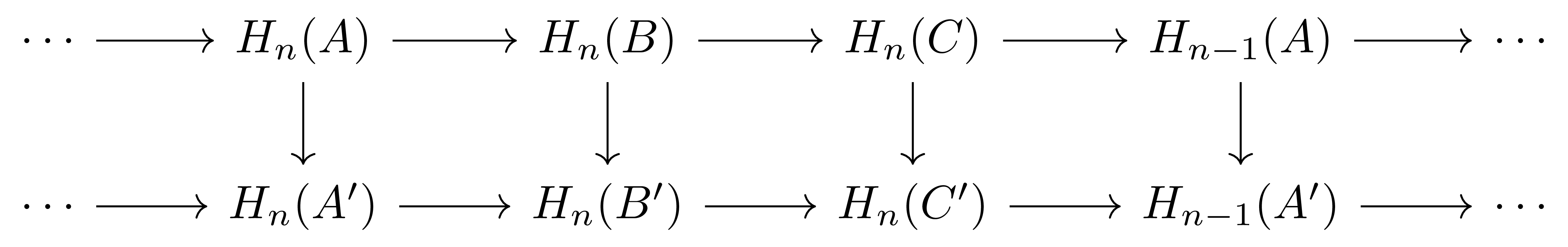
We previously proved that, given any short exact sequence in \(\Ch(\mathcal{A})\)

\[0\longrightarrow A_\bullet\longrightarrow B_\bullet\longrightarrow C_\bullet\longrightarrow 0\]

we can construct the long exact sequence

\[\cdots\rightarrow H_n(A)\rightarrow H_n(B)\rightarrow H_n(C)\rightarrow H_{n-1}(A)\rightarrow \cdots\]

The most essential part of this proof was defining the connecting map \(\delta\), and we generalize this process as follows.

Definition 1 Let two abelian categories \(\mathcal{A},\mathcal{B}\) be given. Then a homological \(\delta\)-functor from \(\mathcal{A}\) to \(\mathcal{B}\) means a collection of additive functors \(T_n:\mathcal{A}\rightarrow\mathcal{B}\) (\(n\geq 0\)), together with morphisms \(\delta_n:T_n(C)\rightarrow T_{n-1}(A)\) defined for every short exact sequence

\[0\longrightarrow A\longrightarrow B\longrightarrow C\longrightarrow 0\]

For \(n<0\), we regard all \(T_n\) as zero. These satisfy the following conditions.

1. (Long exact sequence) The sequence

   \[\cdots\longrightarrow T_{n+1}(C)\overset{\delta}{\longrightarrow}T_n(A)\longrightarrow T_n(B)\longrightarrow T_n(C)\overset{\delta}{\longrightarrow}T_{n-1}(A)\longrightarrow \cdots\]

   is exact.

2. (Naturality) Given a homomorphism between short exact sequences

   

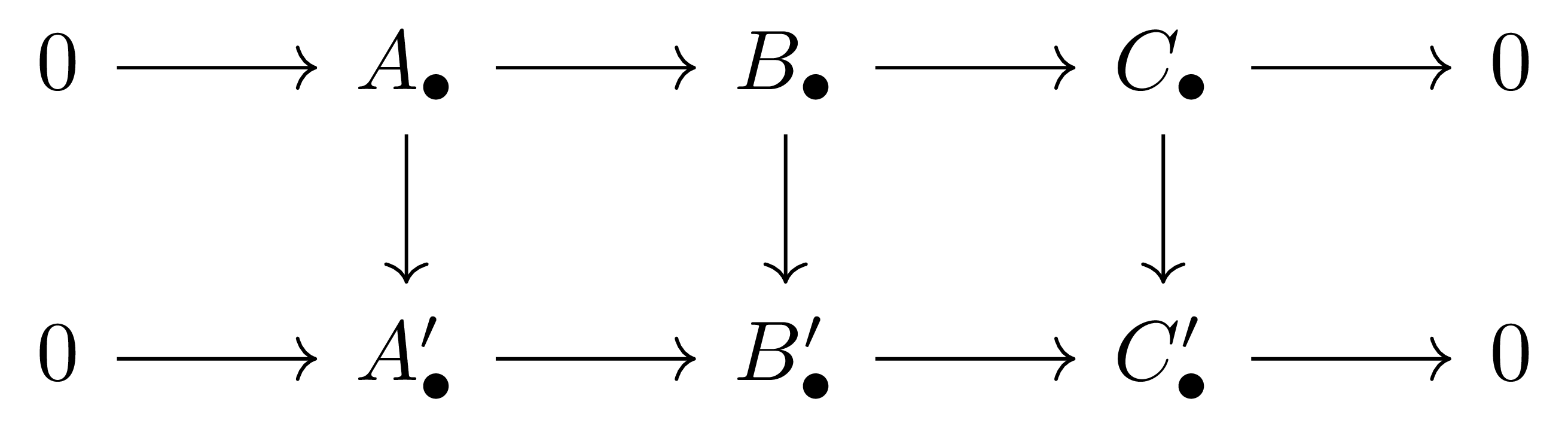
   the following diagram

   

   commutes.

Rewriting the above definition with \(T^n\) and \(\delta^n:T^n(C)\rightarrow T^{n+1}(A)\), we obtain the definition of a cohomological \(\delta\)-functor. Since we have agreed to regard both \(T_n\) and \(T^n\) as zero when \(n<0\), the first condition for a homological \(\delta\)-functor means in particular that

\[\cdots\longrightarrow T_0(A)\longrightarrow T_0(B)\longrightarrow T_0(C)\longrightarrow0\longrightarrow 0\longrightarrow\cdots,\]

that is, \(T_0\) is a right exact functor. Similarly, the first condition for a cohomological \(\delta\)-functor makes \(T^0\) a left exact functor.

Also, the second condition of a \(\delta\)-functor, naturality, means that when we consider the two functors \(T_i(C)\) and \(T_{i-1}(A)\) from the collection of short exact sequences \(\mathbf{S}(\mathcal{A})\) to \(\mathcal{A}\), \(\delta_i\) is a natural transformation between them.

As always, the cohomological case can be easily derived from the homological one, so we shall consider only homological \(\delta\)-functors from now on.

Definition 2 Let two \(\delta\)-functors \(S,T\) be given. Then a morphism \(S\rightarrow T\) means a collection of natural transformations from \(S_n\) to \(T_n\) that commute with \(\delta\).

In other words, it is a collection of natural transformations \(\alpha_n:S_n\Rightarrow T_n\) making the following diagram commute for every short exact sequence

\[0\longrightarrow A\longrightarrow B\longrightarrow C\longrightarrow 0\]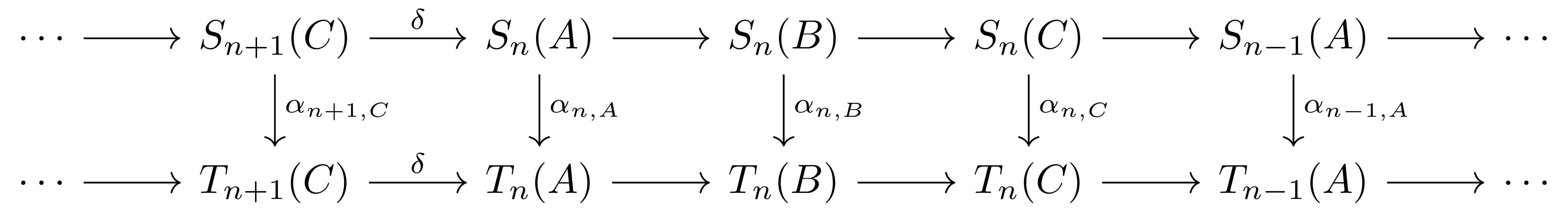

Definition 3 A \(\delta\)-functor \(T\) is called a universal \(\delta\)-functor if, whenever a \(\delta\)-functor \(S\) and a natural transformation \(\alpha_0:S_0\rightarrow T_0\) are given, there exists a unique morphism \((\alpha_n:S_n\Rightarrow T_n)\) of \(\delta\)-functors extending it.

Derived Functors

Consider a right exact functor \(F: \mathcal{A}\rightarrow \mathcal{B}\) between two abelian categories \(\mathcal{A}\) and \(\mathcal{B}\). Then \(F\) does not preserve left exactness. For example, if \(F\) is a covariant functor, then even when the following short exact sequence

\[0 \rightarrow A_1 \rightarrow A_2 \rightarrow A_3 \rightarrow 0\]

is given, only the exactness of the sequence

\[F(A_1) \rightarrow F(A_2) \rightarrow F(A_3)\rightarrow 0\]

is preserved. Likewise, a left exact functor does not preserve right exactness.

The philosophy of derived functors is to supplement the information lost on the left or the right by using infinitely many terms. Thus, for a right exact functor \(F\), our goal is to find homological \(\delta\)-functors satisfying \(T_0=F\), and similarly for a left exact functor, our goal is to find cohomological \(\delta\)-functors.

Definition 4 Let a right exact functor \(F:\mathcal{A}\rightarrow \mathcal{B}\) be given, and suppose \(\mathcal{A}\) has enough projectives. Then the left derived functors \(L_iF\) of \(F\) are defined by the formula

\[(L_iF)(A)=H_i(F(P_\bullet)),\qquad\text{$P_\bullet$ a projective resolution of $A$}\]

For this definition to make sense, \(L_iF(A)\) must not depend on the choice of \(P_\bullet\) made above.

Lemma 5 \(L_iF(A)\) does not depend on the choice of \(P_\bullet\) above.

Proof

Take two projective resolutions and apply §Resolutions, ⁋Theorem 6 to the identity map.

Now let us examine left derived functors in more detail. First, since \(F\) is right exact, we know that the following sequence

\[F(P_1) \overset{Fd_1}{\longrightarrow} F(P_0) \overset{F\epsilon_0}{\longrightarrow} F(A) \longrightarrow 0\]

is exact. Therefore, we obtain

\[L_0F(A)=H_i(F(P))=\frac{F(P_0)}{\im Fd_1}=\frac{F(P_0)}{\ker F\epsilon_0}\cong F(A)\]

To show that the \(L_\bullet F\) form a homological \(\delta\)-functor, we must first show that they are additive functors, and then construct the connecting maps \(\delta\). We divide this into two steps.

Lemma 6 The \(L_iF\) are additive functors.

Proof

First, given any \(f: A' \rightarrow A\) and projective resolutions of \(A'\) and \(A\) respectively, we can apply §Resolutions, ⁋Theorem 6 to obtain \(L_nF(f)\). That this satisfies functoriality and additivity is obvious from the universal property.

Lemma 7 The \(L_iF\) form a homological \(\delta\)-functor.

Proof

First, suppose a short exact sequence

\[0 \rightarrow A \rightarrow B \rightarrow C \rightarrow 0\]

is given. If projective resolutions \(P_\bullet\) of \(A\) and \(R_\bullet\) of \(C\) are given, then using §Resolutions, ⁋Lemma 7 we obtain a projective resolution \(Q_\bullet \rightarrow B\). On the other hand, since each \(R_n\) is projective, the sequence

\[0 \rightarrow P_n \rightarrow Q_n \rightarrow R_n \rightarrow 0\]

is split exact. From this,

\[0 \rightarrow F(P_\bullet) \rightarrow F(Q_\bullet) \rightarrow F(R_\bullet) \rightarrow 0\]

is also a short exact sequence ([Multilinear Algebra] §Hom and Tensor Products, ⁋Proposition 1), and considering the homology sequence here, we obtain the desired connecting maps and the long exact sequence of left derived functors

\[\cdots\overset{\partial}{\longrightarrow}L_iF(A')\longrightarrow L_iF(A)\longrightarrow L_iF(A'')\overset{\partial}{\longrightarrow}L_{i-1}F(A')\longrightarrow L_{i-1}F(A)\longrightarrow L_iF(A'')\overset{\partial}{\longrightarrow}\cdots\]

That the information thus obtained satisfies the second condition of Definition 1 follows from §Resolutions, ⁋Theorem 6.

Moreover, they define a universal homological \(\delta\)-functor in the sense of Definition 3. We omit the proof of this.

Proposition 8 Consider an abelian category \(\mathcal{A}\) with enough projectives and any right exact functor \(F: \mathcal{A}\rightarrow \mathcal{B}\). Then the derived functors \(L_nF\) are universal \(\delta\)-functors.

Just as in the discussion above, we can also define right derived functors for a left exact functor. Its definition is the “dual” of Definition 4.

Definition 9 Let a left exact functor \(F:\mathcal{A}\rightarrow \mathcal{B}\) be given, and suppose \(\mathcal{A}\) has enough injectives. Then the right derived functors \(R^i F\) of \(F\) are defined by the formula

\[(R^iF)(A)=H_i(F(I^\bullet)),\qquad\text{$I^\bullet$ an injective resolution of $A$}\]

Then one can also show that these are universal cohomological \(\delta\)-functors. The reason we use superscripts, unlike in Definition 4, is that these are literally cohomological \(\delta\)-functors, and they arise mainly when dealing with things related to cohomology.